Figure 1 - Mid - The Navigation and Visualisation of Environmental Audio using Zooming Spectrograms
Other figures that are a part of this publication include: Figure 1 - Top, Figure 1 - Mid, Figure - 4 (Focused stack), and Interactive zooming demo
Fig. 1 - Mid. An acoustic day in the life of the Australian bush as revealed in a false-color 24-hour spectrogram. This image was constructed by combining the spectrograms of three different acoustic indices in RGB colour. For more detail see: Towsey et al., Visualization of long-duration acoustic recordings of the environment, presented at the The International Conference on Computational Science (ICCS 2014), Cairns, Australia, 2014.
A 24-hour false-colour spectrogram produced by mapping the indices BGN-POW-CVR to red-green-blue respectively.
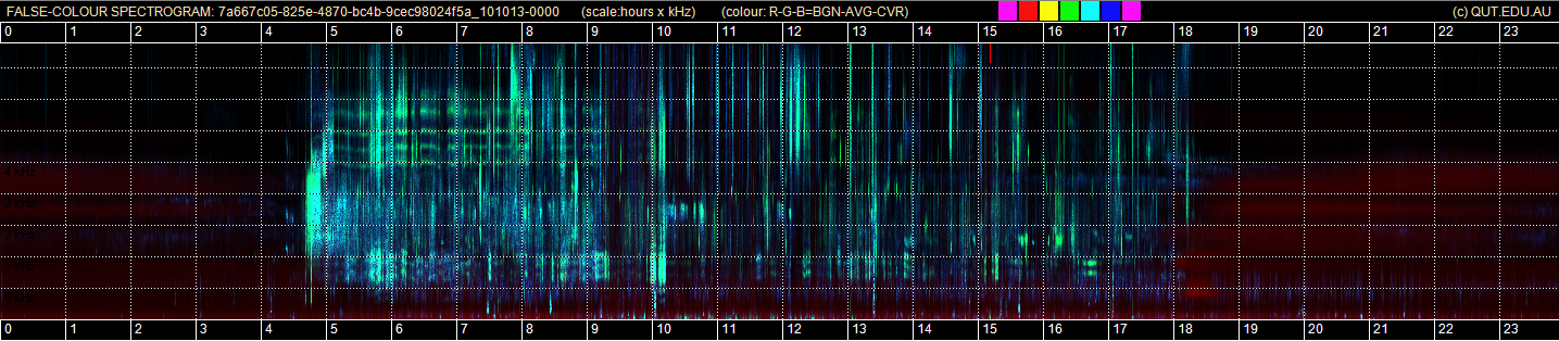
Axes: Vertical grid-lines are at one hour intervals, starting and ending on midnight. The horizontal grid-lines are at 1 kHz intervals.
Hover over the descriptions below to highlight sections of the image.
- Morning Chorus
- Crickets - Orthoptera - four frequency tracks of four species, flat because not temperature sensitive.
- Crows - Corvus orru - note that the stacked harmonics are not as clear as in the ACI-ENT-EVN spectrogram.
- Grey Fantail - Rhipidura albiscapa
- Yellow-faced Honeyeater - Lichenostomus chrysops - poorly distinguished compared to ACI-ENT-EVN spectrogram.
- Olive-backed Oriole - Oriolus sagittatus
- Striated Pardalote - Pardalotus striatus - poorly distinguished compared to ACI-ENT-EVN spectrogram.
- Wind gusts, mild
- Dog barking intermittently - poorly visible compared to ACI-ENT-EVN spectrogram.
- Cicada chorus - visible with this combination of indices but not visible when indices ACI, ENT and EVN are combined.