Preface
This page is an adaptation of a presentation produced by Michael Towsey that was given to various external research groups in February and March 2016. It is a good summary of our current research.
You can contact Michael or our research group by going to the contact us page.
Contents
- Slide 1: Introduction
- Slide 2: The Standard Spectrogram
- Slide 3: Long-duration spectrograms
- Slide 4: Different indices give different views
- Slide 5: Long-duration, false-colour spectrograms
- Slide 6: The utility of long-duration, false-colour spectrograms
- Slide 7: The right combination of indices is important
- Slide 8: Biophony
- Slide 9: Geophony
- Slide 10: Anthropophony
- Slide 11: Adelbert Ranges, Papua New Guinea
- Slide 12: Sturt National Park
- Slide 13: Cross-site comparison (varying latitudes)
- Slide 14: Cross-site comparison (varying altitudes)
- Slide 15: Fresh water recordings
- Slide 16: Marine recordings
- Slide 17: 44 days of ocean recordings
- Slide 18: 44 days of ocean recordings – with sunrise, sunset, and tidal annotations
- Slide 19: Terrestrial ribbon plots
- Slide 20: Diel plots - illustrating four months of acoustic recording
- Slide 21: Diel plots - illustrating thirteen months of acoustic recording
- Slide 22: Comparing soundscapes
- Slide 23: Comparing soundscapes
- Slide 24: Acoustic signatures
- Slide 25: Two acoustic disciplines: Bio-acoustics and Eco-acoustics
- Bridging the divide between bioacoustics and eco-acoustics
- Conclusion
- References
Slide 1: Introduction
Slide 1.
This presentation describes work being done in the Ecoacoustics Laboratory at the Queensland University of Technology (QUT). An important part of our research is the visualisation, navigation, and analysis of long-duration recordings of the environment. Recordings of the environment help ecologists to monitor species diversity, endangered species, and the effects of climate change. It is fortunate that three major groups of vocal animals, birds, frogs, and insects, are also good indicators of environmental health. Acoustic recordings can therefore help in long term studies of environmental change, whether due to negative factors such as pollution, habitat loss, climate change, or due to positive factors such as conservation and restoration projects.
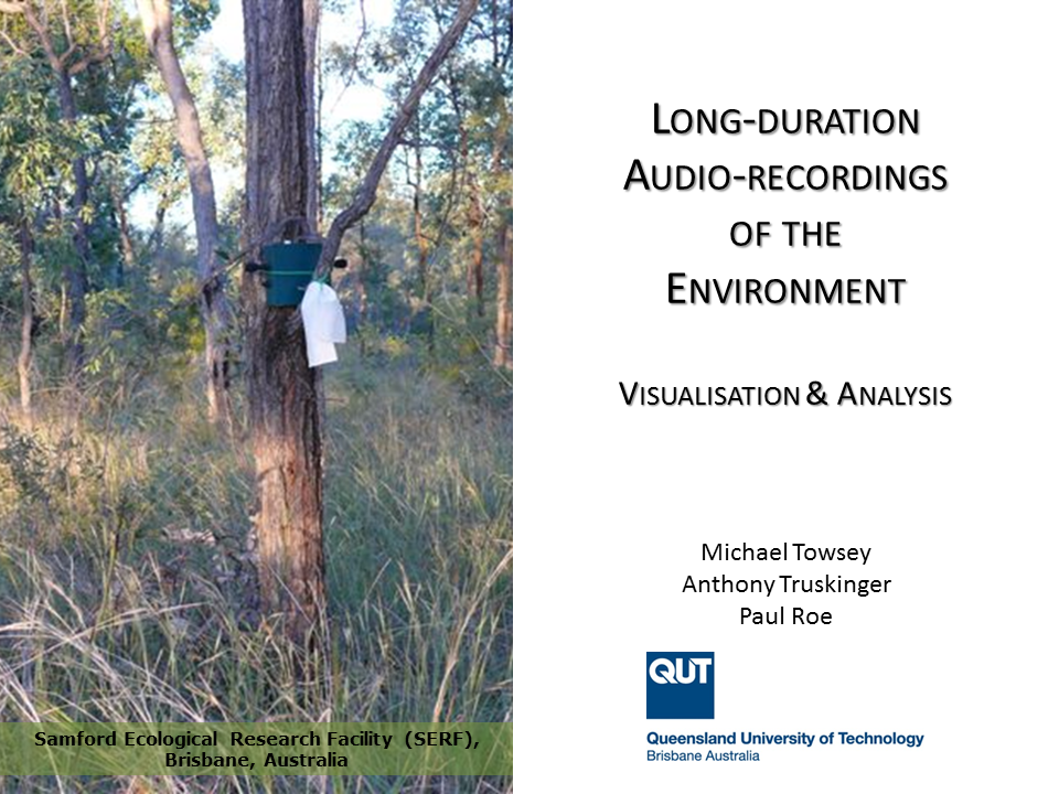
The above image shows a sound recording unit attached to a tree in bushland at the Samford Ecological Research Facility (SERF), on the outskirts of Brisbane City. Most of our recordings are obtained using SM2/SM4 recording boxes manufactured by Wild Life Acoustics, Massachusetts (as in the above image) or BAR recording boxes manufactured by Frontier Laboratories, Brisbane.
Slide 2: The Standard Spectrogram

Slide 2.
A short snippet of the Lewins Rail on the edges of Brisbane City
Ecologists have long worked with spectrograms, two dimensional representations of sound, with time as the x-axis and frequency (Hertz or kilohertz) as the y-axis. Sound amplitude is coded by the grey-scale intensity. The typical spectrogram will be a few seconds long, or as long as required to demonstrate the animal call of interest. We have used acoustic recordings to monitor the cryptic Lewins Rail on the edges of Brisbane City. The sounds at 8 kHz and above in the spectrogram are due to crickets. There are at least four other birds also calling. However, if we want to prepare a spectrogram of a 24-hour recording at similar scale to that shown in Slide 2, it would require a computer screen 1.2 kilometres wide!
An additional problem with acoustic recordings is that technological advances now make it possible to record days, months, or even years of audio–far in excess of what can ever be listened to. Clearly some kind of audio reduction is required. Visualisation of sound is a promising approach because, of all the human senses, the visual sense has the greatest capacity to synthesise and integrate large amounts of information.
Slide 3: Long-duration spectrograms
Slide 3.
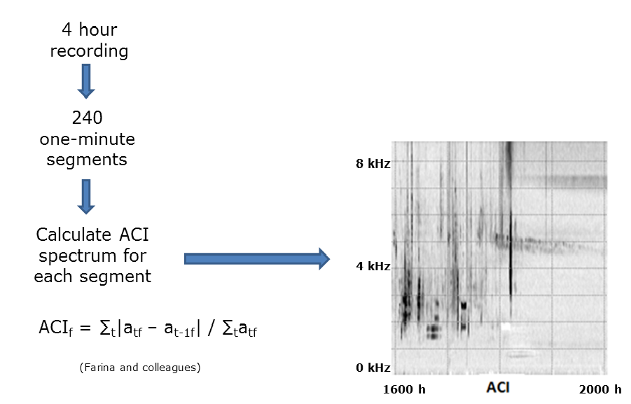
A good way to reduce the information in acoustic recordings of the environment is by using acoustic indices. An acoustic index can be understood as a statistic, that is, a single value to summarise some aspect of the distribution of acoustic energy in a recording. Just as weather reports give average temperature to summarise the weather over an entire day, so we can also use acoustic indices to summarise acoustic properties in a segment of recording.
There are now a lot of studies [see for example the papers of Almo Farina (Italy), Jerome Sueur (France), Stuart Gage (USA) and their students who collectively developed this field of research] which shows that certain indices such as the Acoustic Complexity Index (ACI)1 can detect the presence of biological sounds but remain unresponsive to various kinds of monotonous machine noise. This is useful when one wishes to characterise sound in a semi-urban environment. ACI measures the amount of relative change in sound amplitude from one time instant to the next.
It is possible therefore to prepare a spectrogram of a long duration recording using just the ACI index. We illustrate the method using a four-hour recording (4-8pm) obtained 10th October 2013. (See Slide 3). We break the four-hour recording into 240 one-minute segments. We prepare a standard spectrogram for each one-minute of recording and then calculate the ACI value for each of its 256 frequency bins. Each minute of recording therefore yields a single ACI spectrum containing 256 values. We then join the 240 spectra to make a spectrogram. As illustrated in Slide 3, the ACI spectrogram reveals a lot of acoustic structure. For example, the two tracks after sunset (right side of the spectrogram) are due to the chirps of two different species of cricket–note how the tracks decrease in frequency as temperature declines with the onset of night. Other dominant features in the spectrogram are due to birds.
Slide 4: Different indices give different views
Slide 4.
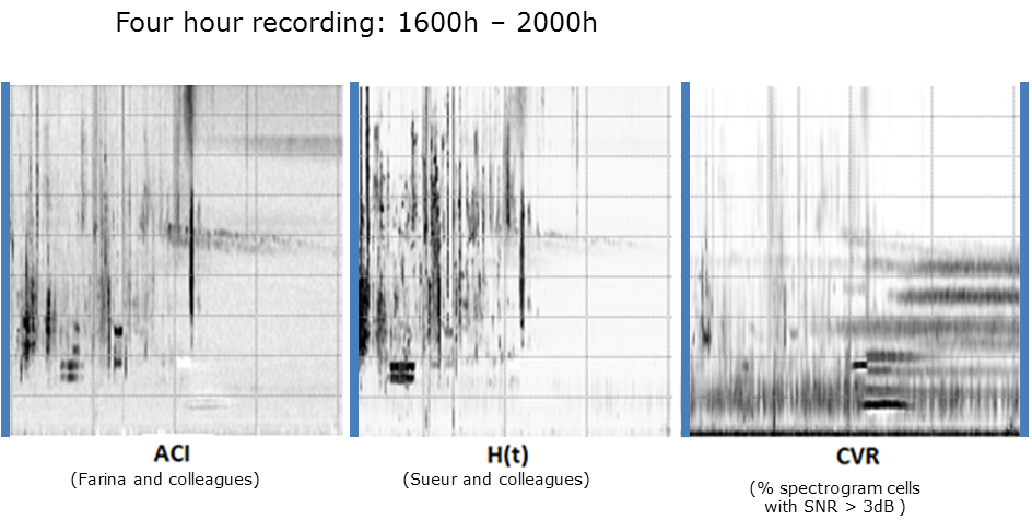
In like manner, we can make additional spectrograms derived from other acoustic indices. In fact, one can experiment with many kinds of index in order to reveal the acoustic structure of interest. In this image, you see long-duration spectrograms prepared from three different acoustic indices. The H(t) index refers to temporal entropy. It measures the degree of (temporal) concentration of acoustic energy in a frequency bin. With continuous background noise, the acoustic energy is highly dispersed, yielding a low value for H(t). If the only sound over the minute is a single dog bark, the sound is concentrated and the value of H(t) will be high.
CVR is short for cover. It simply measures the fraction of spectrogram cells in a given frequency bin where the acoustic energy exceeds a threshold, typically 3 decibels (dB). These are comparatively simple indices, but the important point to note is that each index reveals different components or events in the acoustic sound-space. For example, a 30-minute cicada chorus is only seen in the CVR spectrogram starting at 6pm at 900 Hz. A strong event is shown at 4:30pm (1.8 kHz) in the H(t) spectrogram which is not so obvious in the other spectrograms.
We have now introduced two new terms, sound-space and acoustic event. Sound-space is the abstract notion of a space with five-dimensions, one of time, one of frequency and three of physical space. It is the “space” in which acoustic events occur. An acoustic event is typically a single uninterrupted sound that can be attributed to the same source. The source might be single animal or a chorus of many animals (such as cicadas). A spectrogram reveals the distribution of acoustic energy in the time-frequency dimensions for a fixed point in space. (See Towsey, 20172 for an account of how we calculate many acoustic indices.)
Slide 5: Long-duration, false-colour spectrograms
Slide 5.
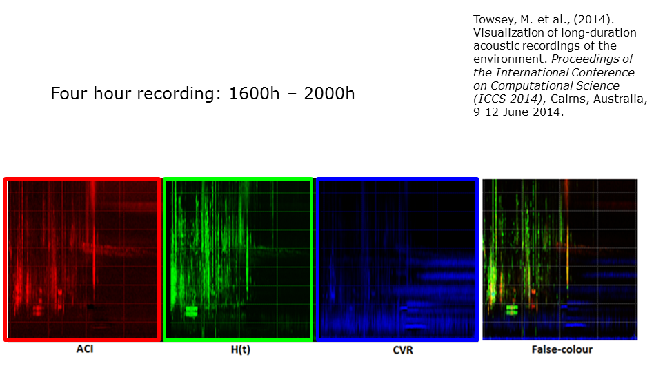
The next step in the production of long duration spectrograms was inspired by false-colour satellite imagery in which pictures of the earth’s surface are rendered in three colours by assigning the red, green and blue (RGB) colours to sensors that respond to different parts of the electromagnetic spectrum. In this case we assign RGB to the three different spectrograms and thereby produce the long-duration, false-colour spectrogram seen on the right-hand side of this slide3. Note how the complexity of acoustic structure in the sound-space is clearly revealed.
Slide 6: The utility of long-duration, false-colour spectrograms
Here we see just how much extra acoustic structure can be seen in a false-colour spectrogram. We took a full 24-hour recording (starting at midnight and finishing the following midnight – this is the same recording from which the 4 hours of the previous slides were extracted) and processed them using a standard audio software tool (Audacity) and our false-colour technique. Ordinarily you would not ask Audacity to open a 24-hour recording but it can be done (with a lot of patience!) on a high performance computer. Audacity achieves the 3000-fold reduction by averaging over long segments of recording. However this smooths out the acoustic structure and makes most events invisible.
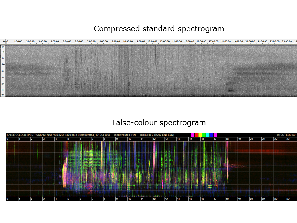
Slide 6.
The basic structure of the forest soundscape at SERF is easily interpreted. (Soundscape is a new word – it refers to the collectivity of acoustic events that occur in a sound-space. It is analogous to landscape in three dimensional space.) The morning chorus is clearly visible at 4:45am. It tends towards white in colour because all indices have high values. The onset of evening is indicated by the onset of acoustic tracks due to insects. But clearly there are many other events.
A colour chart is added at the top of the image to help with interpretation. For example, purple events have high values for ACI and CVR. Cyan events have high values for H(t) and CVR. This will depend on the characteristic distribution of acoustic energy in the animal calls that contribute to the event. With some experience you begin to recognise the different sounds of interest.
For convenience, we refer to these spectrograms as long-duration, false-colour spectrograms or LDFC spectrograms.
Slide 7: The right combination of indices is important

Slide 7.
Different combinations of indices give different views of the soundscape. Here we see two LDFC spectrograms of the same recording. Note that more acoustic structure is visible in the bottom spectrogram than in the top, because two of the three indices used to construct the top spectrogram are correlated. So here we have an important “trick” in making this technique work. Each of the three indices used to construct an LDFC spectrogram should be independent of each other – or at least have the minimum correlation possible. In the top image the two indices AVG and CVR are highly correlated and therefore the third index (CVR) is not adding any new information to the other two. The EVN index in the second spectrogram is a measure of the acoustic events per second in each frequency bin.
Slide 8: Biophony
(Biophony is a new word. It is used by soundscape ecologists to refer to sounds of biological origin - usually bird, insect, frog and mammal calls.)
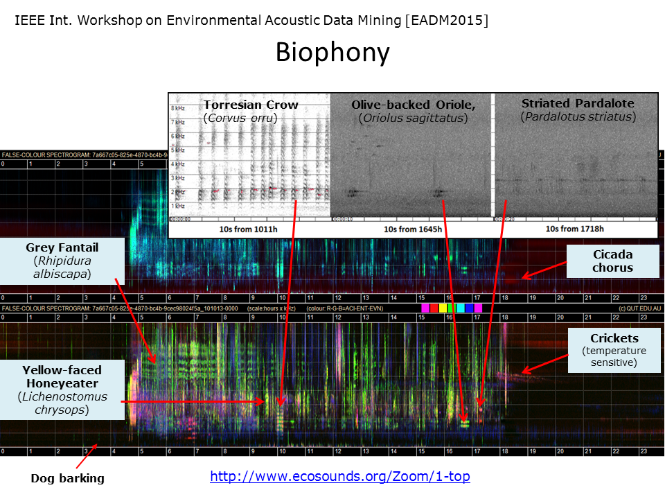
Slide 8.
In this slide, we identify some of the birds that produced the acoustic events in the two spectrograms. While the top spectrogram is not as informative, it does show up the cicada chorus at 6pm. Note that much of the structure in these images comes about because a bird (or birds) tends to sit in the same tree for a few minutes and is likely to repeat the same song/call. Even though a bird may only call once or twice in a minute, one or other acoustic index will “detect” the call and calls over consecutive minutes will leave a clearly visible trace in the spectrogram. Note that these false-colour spectrograms were not designed to identify bird species. The fact that this is possible is “icing-on-the-cake”.
You can see an interactive version of this slide here.
Slide 9: Geophony
(Geophony refers to sounds of natural, but inanimate origin, - usually rain, thunder, wind, surf, etc.)
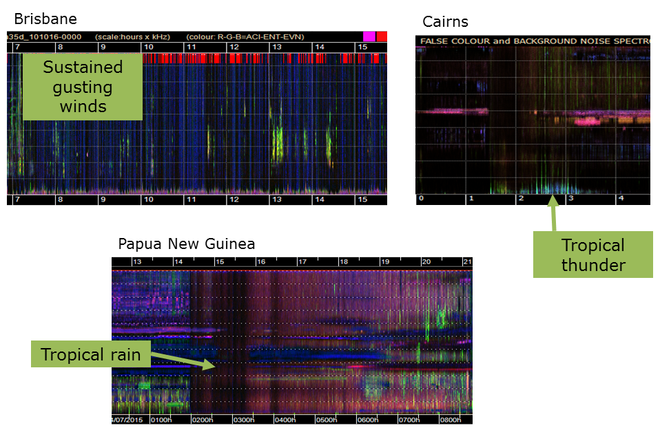
Slide 9.
The typical soundscape will be filled with sounds from many different sources, not just from animals. Soundscape ecologists broadly categorise three or four sound sources which they label, biophony, geophony, anthropophony and sometimes a fourth is added, technophony (to distinguish musical sounds and speech from machine noise). In the above three LDFC spectrograms, we see traces left by various kinds of geophony. In the top-left spectrogram, note that bird song (in green) occurs in between gusts of wind (in blue). A spectrogram like this can direct an ecologist to those parts of the recording in which birds are singing, thereby saving a lot of time.
The traces left by rain in an LDFC spectrogram can vary a lot, obviously depending on the rain intensity but also on local characteristics, such as leaf size, leaf litter and even the acoustic response of the recording box to the percussive effects of rain drops
Slide 10: Anthropophony
(Anthropophony refers to sounds caused by humans, everything from speech and music, to machine noise emanating from planes, trains, bikes and automobiles. Machine noise is sometimes called technophony.)
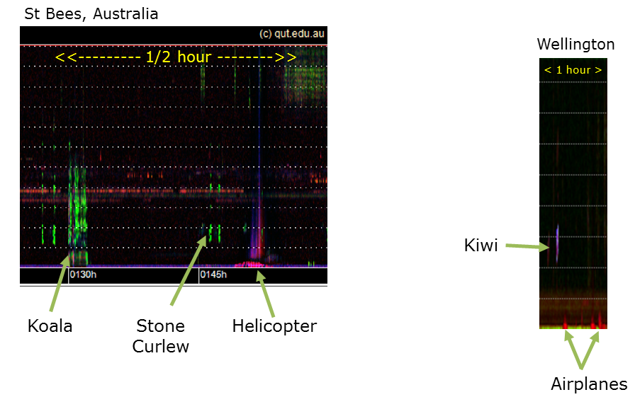
Slide 10.
These images show two sources of anthropophony/technophony due to planes and a helicopter. Plane noise is typically in the low frequency band. It has a pyramid shape in the spectrogram, due to the fact that low frequency sounds travel further than high frequency sounds. As a plane approaches the microphone, the low frequency sounds are detected first and the high frequency sounds are heard only when the plane is closer. The reverse happens as the plane flies away. The speed and distance of the plane can be determined from the shape of the pyramid. Note the dual components of helicopter noise, a low frequency component due to the engine and a high frequency component due to the whipping of the rotors.
Anthropophony is a frequent problem for ecologists wanting to record only animal calls. The above images also illustrate the sounds of a koala, stone curlew and kiwi. Here is recording of a koala bellow.
This recording has a Koala call in it.
Slide 11: Adelbert Ranges, Papua New Guinea
This LDFC spectrogram was obtained from the Adelbert Ranges, Papua New Guinea, by The Nature Conservancy (TNC). TNC is a global conservation organisation who are attempting to preserve some of the natural forests of PNG. See more info on the Adelbert Mountains project here and here.
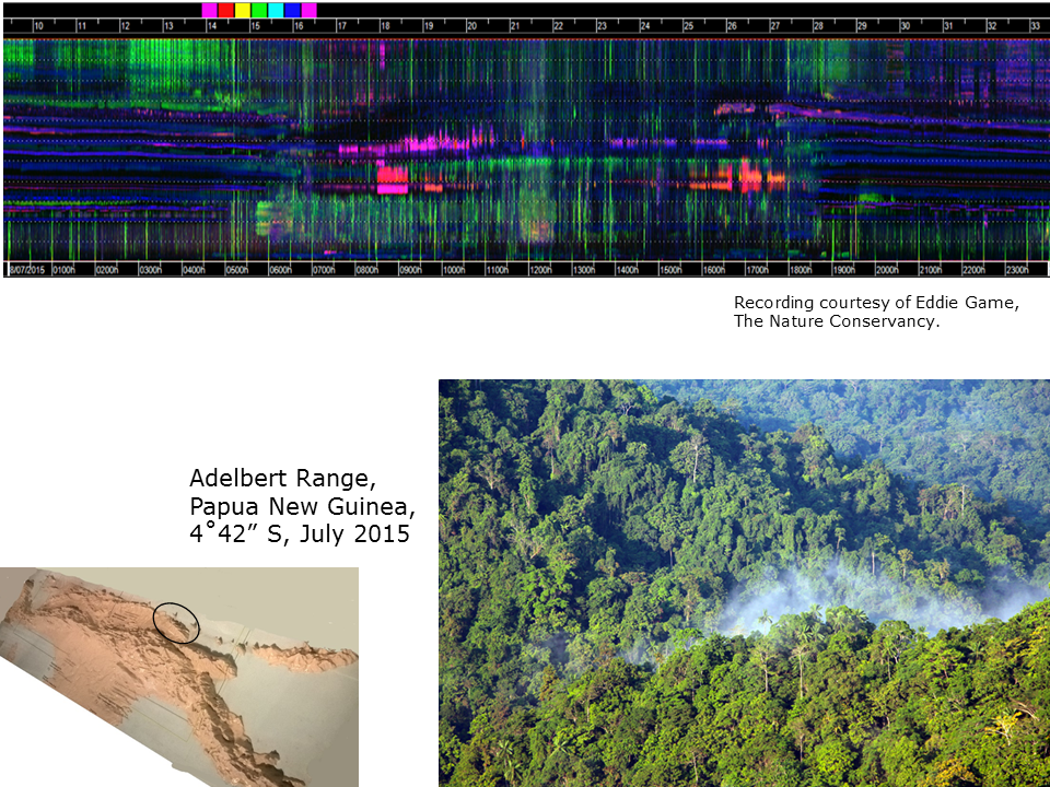
Slide 11. Audio courtesy of Eddie Game and the Nature Conservancy
The local terrain for this recording is mountainous jungle. Note how the entire sound-space is filled with acoustic activity, most of it due to insects. Birds are, for the most part, restricted to the lower frequency band. The morning chorus is not as well-defined as in the previous recording from eucalypt woodland in Australia. It is difficult to imagine how you could cram another vocal species into this sound-space! This brings us to the notion of the sound-space as a finite ecological resource. Somehow all the insects, birds and frogs at this location have to partition their acoustic activity in a way that allows them to complete their life-cycles, i.e. so that the mating pairs of each species can find each other in a cacophony of noise.
Slide 12: Sturt National Park
By way of a complete contrast to the previous spectrogram, here is a 24-hour LDFC spectrogram of a semi-desert environment in the Sturt National Park, about 1200 km inland from Brisbane, Australia. (See the semi-desert landscape in bottom image.) Note the highly attenuated morning chorus around 7am, the almost complete absence of sound at night when the winter temperatures are likely to be below freezing, and the gusting winds in the middle of the day (insufficient baffles on the microphones!). There are occasional bird calls at night – see 2040h. This shows once again the utility of the H(t) index in picking out brief bursts of sound in long periods of silence.
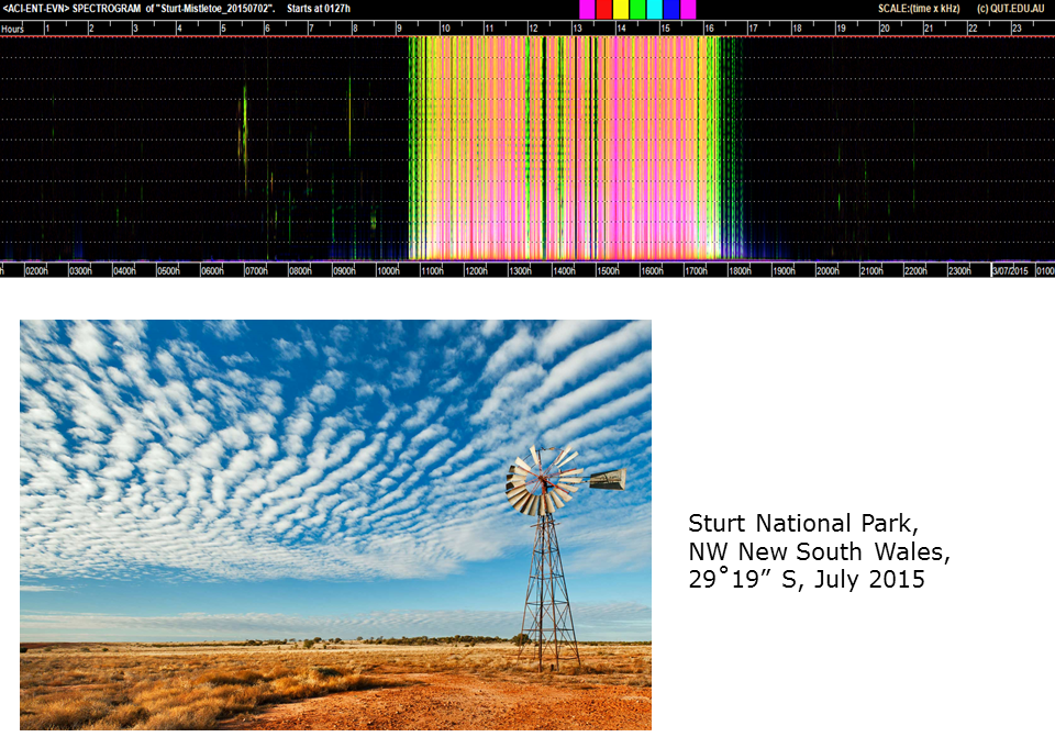
Slide 12. Audio courtesy of Dave Watson.
For more information on the ongoing Sturt National Park acoustics project contact Prof. David Watson from Charles Sturt University (@D0CT0R_Dave).
Slide 13: Cross-site comparison (varying latitudes)
This slide compares three 24-hour, false-colour spectrograms of three soundscapes from different latitudes. All these recordings were obtained in the first week of July (winter) 2015. The top PNG recording is dominated by insects. The middle Brisbane recording is dominated by birds and the bottom desert recording is dominated by wind.
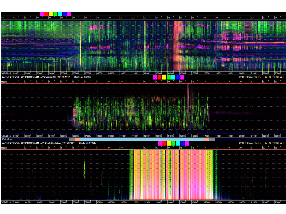
Slide 13.
Recordings courtesy of:
- (top) Eddie Game, The Nature Conservancy
- (middle) Yvonne Phillips, QUT Ecoacoustics Research Group
- (bottom) David Watson, Charles Sturt University
Slide 14: Cross-site comparison (varying altitudes)
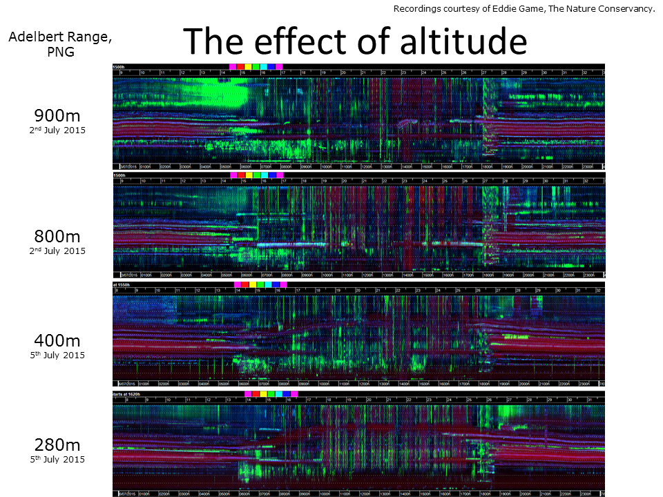
Slide 14. The effect of altitude on sound-scapes as rendered in LDFC spectrograms. Audio courtesy of Eddie Game and the Nature Conservancy.
This slide compares LDFC spectrograms from four Adelbert Range locations that are quite close but differ in altitude. Several differences are apparent, particularly in the 0-2 kHz band. At 280 metres there is a lot of background noise (red colour) in the 0-2 kHz band, whereas at 900m there is more bird activity. Spectrograms such as these can help ecologists to spot differences between recording sites and to frame interesting hypotheses.
Slide 15: Fresh water recordings
Slide 15. Audio courtesy of courtesy of Simon Linke and Toby Gifford.
Not many people know that fish make a lot of sound as do underwater insects and crustaceans. This slide shows two LDFC spectrograms of a 24-hour recording taken with a hydrophone in a pond of the Einasleigh River, northern Queensland, dry season. Note the change in sound during the day compared to the night. All the acoustic activity in this recording is due to aquatic insects and is dominant in the 1-2 kHz band. You can listen to 21 seconds of underwater recording here - all the sound is due to insects.
This recording (courtesy of Simon Linke) shows acoustic activity in a pond in northern Queensland.
The audio shown here was provided by Dr. Simon Linke and Dr. Toby Gifford, of Griffith University, Brisbane, Australia. If you’d like more information on their project please contact them.
Slide 16: Marine recordings
These LDFC spectrograms are derived from a 24-hour hydrophone recording taken 15 km off the coast of Georgia, USA. The water is only 15 m deep and the hydrophone was positioned 2m off the ocean floor. Note in this case, that the horizontal grid-lines are 200 Hz apart with 1 kHz full scale.

Slide 16. Audio courtesy of courtesy of Aaron Rice, Cornell Lab of Ornithology.
The red events in the bottom spectrogram are due to passing ships. Sound can travel long distances underwater and the passage of a ship can be acoustically evident for two or more hours. Note the tendency to “pyramid shape events” because low frequencies travel further than high. In the second ship from the left, you can observe interesting interference effects due to a phenomenon called Lloyd’s Mirror. Sound arriving at the microphone comes directly from the ship but also comes indirectly after reflection at the ocean surface. Interference effects result because the two sound paths have slightly different lengths. Each ship has a different acoustic signature that depends on its depth in the water, propulsion mechanism and noises from inside the ship due to generators and winches.
The dominant bio-acoustic activity in this recording is due to fish clicks at around 100 Hz. However, in many marine recordings of the deep oceans many of the sounds have yet to be identified. Earthquakes and sonar activity (due to military and to oil exploration) also contribute to the marine soundscape. Marine noise pollution is now recognised as a major problem and a contributing factor to whale and dolphin strandings.
The audio provided is courtesy of Aaron Rice, Cornell Lab of Ornithology, Cornell University, NYS, USA.
Slide 17: 44 days of ocean recordings
So far the longest LDFC spectrogram we have viewed is 24-hours long and this takes up the full width of a typical computer screen. In order to view recordings several months long, a different approach must be adopted. The below image represents 44 days of continuous marine recording from the same site as the previous slide. The 24-hour spectrograms have been reduced to a height of 32 pixels but they retain the full 24-hour width. Concatenating the daily spectrograms nicely reveals long-term seasonal acoustic patterns. We call the individual spectrograms, ribbon spectrograms and the total image a ribbon plot.
Slide 17. Audio courtesy of courtesy of Aaron Rice, Cornell Lab of Ornithology.
The noise from passing ships is clearly apparent. The direction, speed and proximity of each ship can be determined by the shape and extension of its pyramid shape. The second dominating component of this sound-scape is the cyan-blue acoustic events at night from day 33 onwards. These are due to the chorusing of the black drum fish. Because of their low frequency, the calls of the black drum fish carry a great distance, even 15 kilometres towards the coast.
A short recording demonstrating dominant acoustic activity in a marine recording off the Georgia Coast, USA. Note the low-frequency noises of the black drum fish (Pogonias cromis). Extract courtesy of Cornell Lab of Ornithology
The third dominating component of this sound-scape occurs during days 9-13. The green lines are due to unidentified “knocking” sounds, something hitting or biting the hydrophone. There were no hurricanes or other meteorological events before or during days 9-13 that might explain these acoustic events. Fishing net strikes are a major problem for marine mammals in the area and may be a possible explanation. However, to get a better understanding of these events, we can add other annotations to the spectrograms as in the next slide.
The audio provided is courtesy of Aaron Rice, Cornell Lab of Ornithology, Cornell University, NYS, USA.
Slide 18: 44 days of ocean recordings – with sunrise, sunset, and tidal annotations
This is the same 44 days of false-colour spectrogram as shown in the previous slide but with sunrise, sunset, high- and low-tide times superimposed. Day length is increasing as the recording proceeds through spring.
Slide 18. Audio courtesy of courtesy of Aaron Rice, Cornell Lab of Ornithology.
While the chorusing of black drum fish is dominant at night and likely to be triggered by increasing day-length, the chorusing does not appear to be constrained by daylight. With respect to the “knocking” sounds in days 9-13, they appear to be at a maximum between low tide and high tide around the new moon, possibly when coastal currents are strongest. We have not been able to identify the cause of this sound. Perhaps they are associated with something drifting in the ocean currents. Or perhaps strong tidal currents cause vibration of the cable tethering the hydrophone to the ocean floor. This is a frequent problem for those recording whale song.
It is worth noting that these hundreds of hours of marine recording were made in order to detect the presence of the North Atlantic Right Whale (NARW), the most threatened of the whale species. The hydrophone was located in the middle of the NARW calving grounds towards the end of the calving season. The usual approach to identifying NARW calls is to write computer programs, specifically designed to recognise the three kinds of NARW call. Due to the highly specific purpose of automated recognisers, they are specially designed not to detect any other acoustic events. However, LDFC spectrograms reveal a wealth of additional information about the marine soundscape. They complement the information obtained by automated call recognisers because they reveal, in much more detail, the acoustic environment in which whales live.
Slide 19: Terrestrial ribbon plots
In the following image, we return to a terrestrial sound-scape, in this case, illustrating 63 days of continuous recording using audio recorded in Gympie National Park, Queensland, Australia.
Slide 19. Audio courtesy of courtesy of Yvonne Phillips, QUT Ecoacoustics Research Group.
The morning and evening choruses are clearly evident as are rain showers shown prominently in red (see ribbon for 21/05/2015). Note how easy it is to compare the structure of the sound-scape over consecutive days. The grey vertical line that appears (typically) every seventh days is when the recorder was turned off in order to change batteries. (Not everything is ecologically significant!)
Slide 20: Diel plots - illustrating four months of acoustic recording

Slide 20. Audio courtesy of courtesy of Yvonne Phillips, QUT Ecoacoustics Research Group.
Even with the ribbon spectrograms reduced to a height of 32 pixels (as in the previous slide), there is a limit to how many ribbons can be concatenated to illustrate many months of recording. In theory we could try reducing each ribbon to a single pixel height, but instead we derive this kind of very-long-duration acoustic image from summary acoustic indices rather than spectral acoustic indices. A summary index (the acoustic bit is assumed) is a single value representing the distribution of acoustic energy in an entire minute of recording over all frequency bands. That is, frequency information is now lost.
In this image (Slide 20), you see a representation of four months of recording, each pixel row representing one day of recording. The left-hand side of the image is midnight, the image-centre represents midday and the right-hand side the following midnight. We call these plots diel plots. The time of civil-dawn and civil-dusk is superimposed. It is obvious that, unlike the previous marine sound-scape, the terrestrial sound-scape is highly constrained by daylight.
To produce this image, the three summary indices assigned to red, green and blue respectively were: 1: an estimate of background noise; 2. the signal-to-noise ratio; and 3. the average number of acoustic events per second. Each of these indices was calculated from the signal wave form. That is, there was no need to do the intermediate step of making a standard spectrogram. The emerging red patches (bottom right) are due to the onset of insect chorusing as spring temperatures increase. The long horizontal lines are due to extended periods of rain. The red patches within the blue lines are due to extremely heavy rain bursts. The morning chorus is clearly aligned with civil-dawn (around 30 minutes before actual sunrise) and the bright-green specks that are most apparent around sunrise and sunset are due to loud kookaburra choruses. Just as with false-colour spectrograms, diel plots derived from different indices provide different views of the sound-scape.
Audio provided courtesy of Yvonne Phillips, QUT Ecoacoustics Research Group. The audio was recorded in Gympie National Park, Queensland, Australia.
Slide 21: Diel plots - illustrating thirteen months of acoustic recording
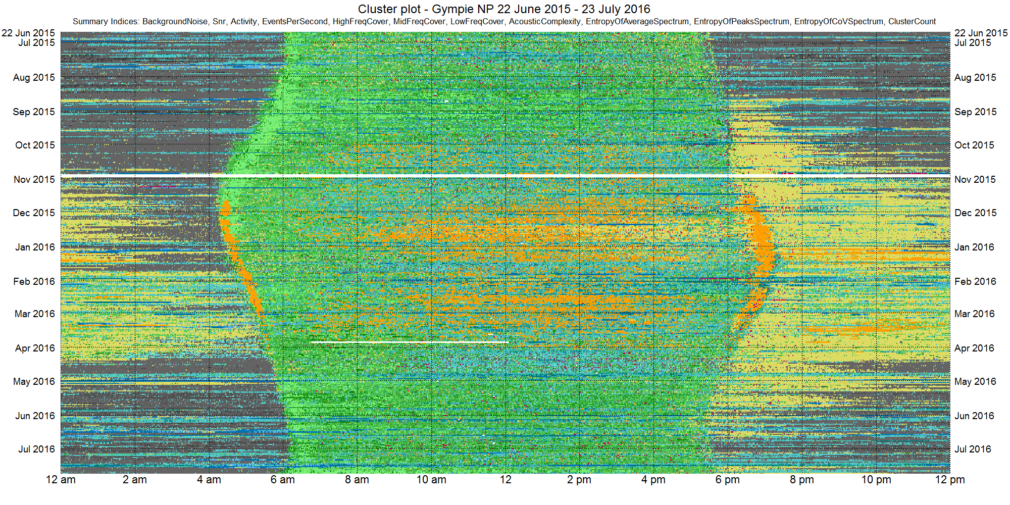
Slide 21. Audio courtesy of courtesy of Yvonne Phillips, QUT Ecoacoustics Research Group.
We have produced diel plots using three different methods. The first way, as illustrated in the previous slide, is to assign three different summary indices to the red, green and blue channels of the image. A second way (not shown in this tutorial) is to calculate several to many summary indices, obtain the first three principal components and assign them to the red, green and blue channels of the image respectively. A third way (illustrated in this image) is to calculate several to many summary indices, cluster them and colour code the resulting clusters. This method is described in Phillips et al. 20174. The above diel plot (Slide 21) was derived from clustering 1.1 million vectors of 12 summary indices. It represents 13 months of continuous audio, recorded in Gympie National Park. Clustering produced 60 clusters (each cluster represents an “environmental acoustic state”) but the colour coding was simplified to seven basic sound categories or acoustic states: 1. silence clusters are represented in grey; 2. bird cluster in green; 3. rain clusters in dark blue; 4. wind clusters in pale blue; 5. insect cluster in yellow; 6. cicada chorus clusters in orange; and 7. plane sounds in red. How the soundscape gradually changes through the seasons is clearly visible.
Audio provided courtesy of Yvonne Phillips, QUT Ecoacoustics Research Group. The audio was recorded from Gympie, Queensland, Australia.
Slide 22: Comparing soundscapes
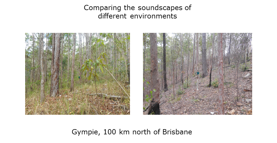
Slide 22. Pictures courtesy of courtesy of Yvonne Phillips, QUT Ecoacoustics Research Group.
By utilising very-long-duration recordings, we are now in a position to make meaningful comparisons between the soundscapes of two locations. For example, consider the two locations shown in this slide (Slide 22). The one on the left (in Woondum National Park) has higher rainfall and smaller temperature fluctuations than the site on the right (in Gympie National Park) because it is closer to the coast. Consequently, the Woondum site supports more dense vegetation cover, yet the bird species are quite similar at the two sites. What are the consequences for the soundscape? How will the soundscapes differ despite similar bird species?
Slide 23: Comparing soundscapes
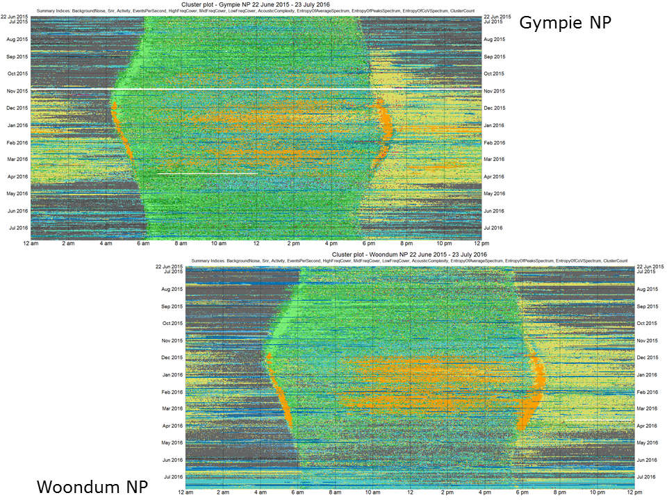
Slide 23. Pictures courtesy of courtesy of Yvonne Phillips, QUT Ecoacoustics Research Group.
This slide (23) illustrates 13 months of soundscape from each of the two locations, Woondum and Gympie National Parks. Taken over the entire year, the soundscapes are similar but have subtle differences. The Gympie site has less cicada activity but more insect activity. We believe that images such as these will be very useful in monitoring the long term effects of climate change. Small but subtle changes in species diversity and ecosystem health will be more likely to be detected when very-long-duration recordings can be compared visually over consecutive years.
Slide 24: Acoustic signatures
.](Slides/Slide26.png)
Slide 24. Sankupellay M., Towsey, M., Truskinger, A., & Roe, P. (2015).
Apart from visualisation, acoustic indices offer other ecological insights. For example, we can classify different locations by deriving “acoustic signatures” from their soundscapes. In one study (Sankupellay et al.5), we selected four sites at one location and two sites at another location. Two consecutive days of recording were made at each of the six sites, giving 12 days of recording in total.
Ten summary acoustic indices were calculated at one-minute resolution over all 12 days (12 × 1440 = 17,280 one-minute recording segments). The vectors of ten indices were normalised and clustered using a 10×10 self-organising map (SOM). The 100 nodes were further clustered to yield 27 clusters, each representing a distinct “acoustic regime”.
The contents of the 27 clusters were identified by selecting the false-colour spectrum of each minute in each cluster (see top image of SLIDE 24). Cluster Y contained very quiet night-time recording segments, while cluster V included the morning chorus and other segments with much bird activity.
A 24-hour cluster occupancy histogram (having 27 bins) was prepared for each of the 12 days (see middle image in slide) and these cluster occupancy histograms were in turn hierarchically clustered. The resulting dendrogram (bottom right image in the slide) clearly shows that the soundscapes of consecutive days at the same site are more similar than those at different sites. The dendrogram also separates the two locations. To sum up, the use of acoustic indices enables the calculation of acoustic signatures that characterise the soundscapes at different locations.
Slide 25: Two acoustic disciplines: Bio-acoustics and Eco-acoustics
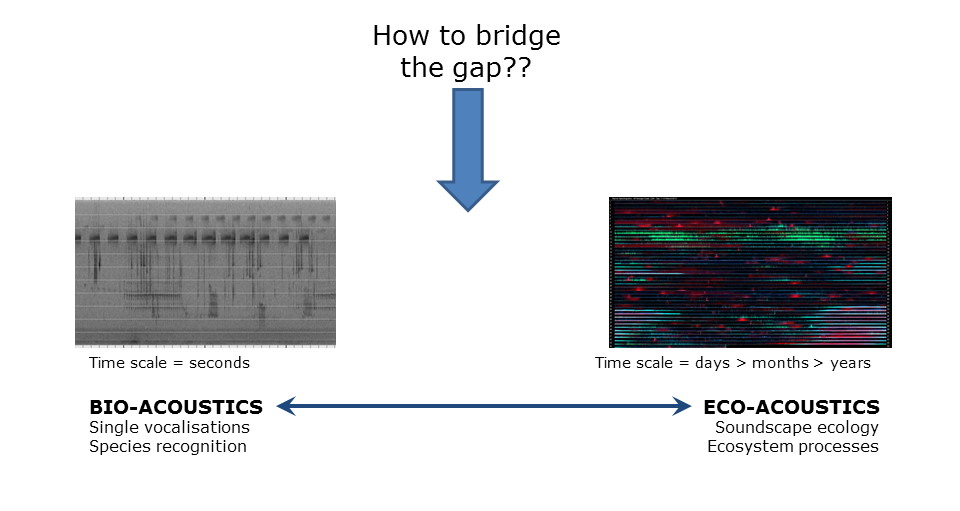
Slide 25.
Until recently, biological interest in acoustics was restricted to the vocalising mechanisms and behaviours of individual animals or species. This science is known as bioacoustics. Technological limitations in previous years did not permit long recordings. However, in the last few years, these technological impediments have pretty much disappeared. The effect has been to open up an entirely new science, which is variously called eco-acoustics or soundscape ecology. Soundscape ecology studies the interactions between soundscapes and the underlying ecosystem processes.
There is a huge (orders of magnitude) difference in the scale of bioacoustics versus eco-acoustics. Bioacoustics studies acoustic phenomena that have only few seconds duration, whereas eco-acoustic patterns may be days, months, or even years in duration. Bioacoustics investigates the behaviour of individuals or single species, whereas eco-acoustics studies, as the name implies, the sounds made by ensembles of thousands of interacting species.
The question arises as to how can we bridge the divide between bioacoustics and eco-acoustics?
In the remaining slides we look at four ways in which work in our lab attempts to bridge this divide.
Bridging the divide between bioacoustics and eco-acoustics
1. Slide 26: Using sound-scape indices to help study species diversity
Slide 26.
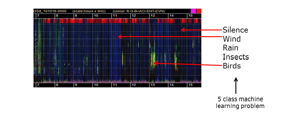
Typically acoustic indices are calculated at one-minute resolution, too coarse a time resolution to be of much interest to bio-acousticians who are interested in animal calls that may last only a few seconds. However acoustic indices can pick up the occurrence of different sounds even if they cannot identify what they are. The spectrogram in Slide 24 is dominated by wind (blue vertical lines) but when the wind drops, birds begin to sing (yellow-green lines). So one use of acoustic indices (calculated at one-minute resolution) is to classify one-minute audio segments according to their general acoustic content. It is relatively easy to construct a five-class machine learning problem where the task is to identify minutes containing bird calls versus silence, wind, rain and insect sounds. The classifier can be used as a filter to remove recording segments that do not contain bird sounds, as shown in the next slide.
](Slides/Slide29.png)
This image (Slide 25) shows a histogram of all the 1440 one-minute segments in one day. The minutes are binned according to how many different bird species are calling in the minute segment. The blue bars indicate the distribution of bird call densities before use of a classifier to filter out non-bird segments. The zero-bird-species bin is by far the largest. The red bars indicate distribution after filtering. The classifier has removed most of the one-minute segments that do not contain bird calls. This means that the ecologist is required to listen to less audio when trying to determine species diversity.
This work in this slide is the research product of Liang Zhang, QUT Ecoacoustics Research Group6.
2. Slide 27: Using acoustic indices to monitor sperm whales

Slide 27. Figure courtesy of Hervé Glotin
Slide 27 shows the Mediterranean Sea and the south coast of France. The city of Toulon is on the left. A few kilometres off the coast, the sea level suddenly drops from 200m to 2000m. The submarine cliff face is carved out by canyons in which sperm whales like to hunt. A hydrophone rig (known as BOMBYX) is placed at the top of one of these canyons. Sperm whales hunt for their prey by emitting sonar clicks and their presence can be detected by identifying clicks at a characteristic periodicity of about one second. You can listen to a short recording of sperm whale clicks here. The first four seconds of the recording are dominated by sonar clicks. When they cease, you can more easily hear the sperm whale clicks.
This recording (courtesy of Hervé Glotin) demonstrates sonar beeps and the clicks produced by a sperm whale (Physeter macrocephalus).
This is typically a problem where code would be written to automate the recognition of sperm whale clicks. Another approach is to calculate generic acoustic indices but this time calculated at 0.1 second resolution rather than one-minute resolution.
The figure is provided by Prof. Hervé Glotin. More information on the BOMBYX project can be found here.
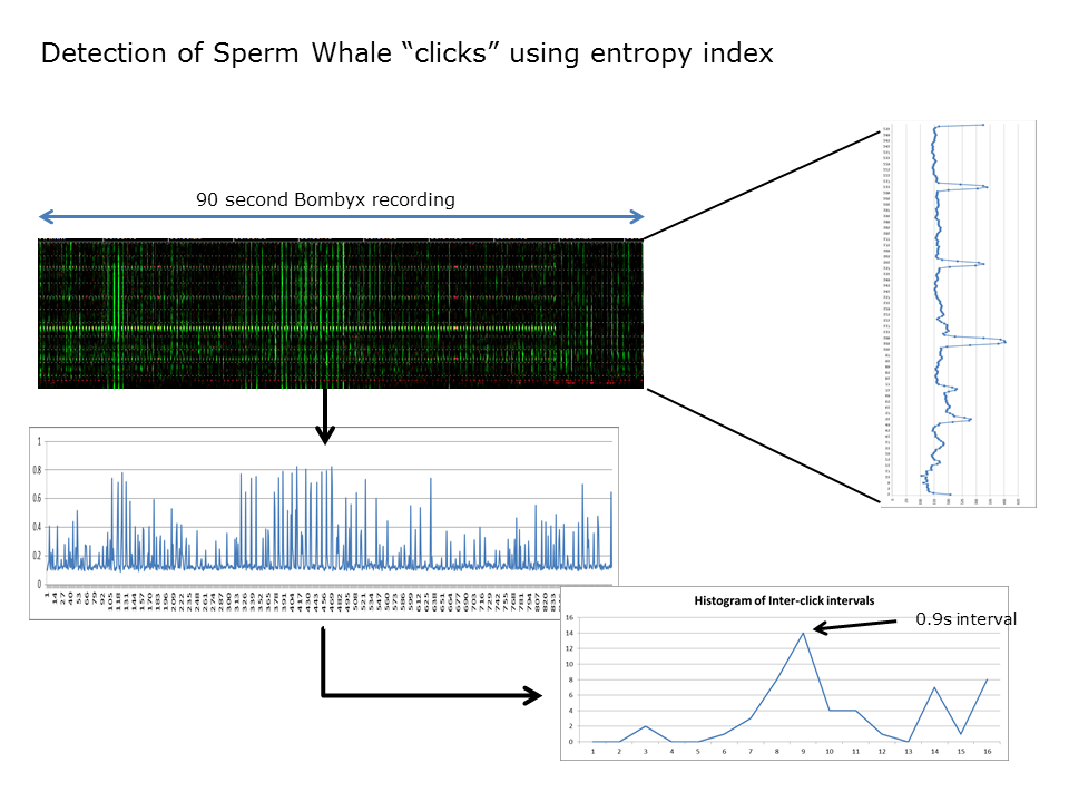
Slide 27.
The generic index which proves to be most useful to detect sperm whale clicks is the temporal entropy index. Slide 27 (top image) shows a spectrogram derived from the H(t) index calculated at 0.1s resolution. The “green” events in the spectrogram are those picked up by H(t). Note that the recording also contains many other “click” sounds, in particular, dominant sonar clicks used to monitor shipping. The sonar clicks must be removed prior to analysis and their harmonics can be easily identified using an averaged spectrum (as shown in top-right image).
The sperm whale clicks are then revealed (centre-left image) and the dominant period between clicks can be shown to be 0.9 seconds (lower-right image). The important idea being demonstrated here is that generic acoustic indices can be used to solve a very specific problem. this makes generic acoustic indices extremely useful.
3. Slide 28: Using acoustic indices for animal welfare
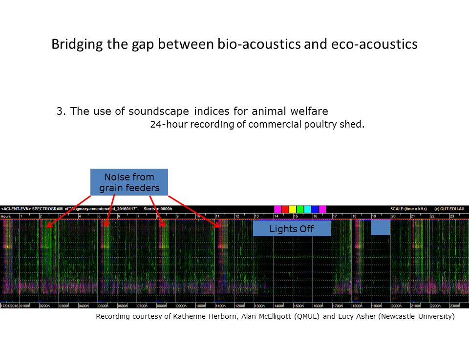
Slide 28. Courtesy of Katherine Herborn, Alan McElligott, and Lucy Asher
The obvious advantages of acoustic approaches to monitor animal behaviour are that recordings are cheap and easy to obtain. They also provide a permanent and objective record. Our lab is working with the University of Newcastle (UK) and Queen Mary University London using acoustics to monitor poultry health. The study involves finding correlations between hen vocalisations and standard measures of animal well-being (e.g. weight loss). The spectrogram in this slide (Slide 28) shows the 24-hour soundscape of a poultry shed. The hens fall silent during “lights-off” but are vocally active with lights on. The dominant vocal band is 1-3 kHz but there is also much activity at high frequencies. Changes in the pattern of calling frequency could provide valuable indicators of poultry health.
Recording courtesy of Dr. Katherine Herborn, Dr. Alan McElligott (QMUL), and Dr. Lucy Asher (Newcastle University).
4. Slide 29: Using acoustic indices at all time-scales
](Slides/Slide35.png)
In previous slides we demonstrated the use of acoustic indices calculated at one-minute resolution to reveal the acoustic structure in a 24-hour soundscape. In Slides 26 and 27, we showed the use of acoustic indices calculated at finer resolution (0.1 seconds) to detect the sonar clicks of a sperm whale. The resolution of a standard spectrogram (as seen for example, in Slide 2) is around 0.01 seconds per frame. In fact it is possible to calculate acoustic indices at multiple time scales and use them to span the entire temporal scale from years and months down to milliseconds. Some indices reveal acoustic structure better at course resolution (for example ACI) and others reveal structure better at fine resolution. We have developed techniques7 in our lab to “stitch” all these different scale images together to make a pyramid stack as shown in Slide 29. But much more useful is that we are now able to “zoom” in and out of long duration recordings in the same way that Google Maps allows you to zoom in and out from planet Earth. This makes it easy to navigate recordings of arbitrary duration. Try a demo of this concept for yourself on a 24-hour recording by going to http://www.ecosounds.org/Zoom/zoom.
We are currently integrating the zooming false colour spectrograms technology into our acoustic workbench software—soon every audio recording hosted on ecosounds.org will benefit from the enhanced visualisation capability of zooming spectrograms.
Conclusion
Slide 30.
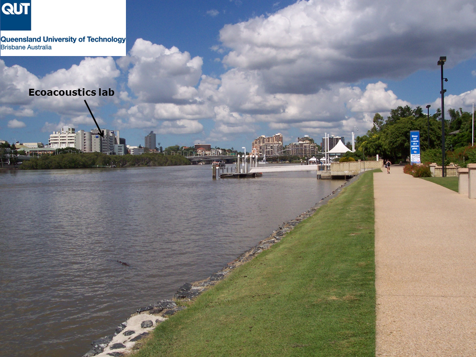
And finally a picture of our lab in the Garden Point campus of the Queensland University of Technology. This picture is taken from across the Brisbane River. Imagine the sounds in this scene. And then consider the submerged soundscape within Brisbane River.
We are at an exciting stage in our research. Ecoacoustics is a rapidly developing field with lots of potential and diverse applications. We tremendously enjoy working with our collaborators. If you see other possible applications for the visualisation and use of acoustic recordings, go to our contact page .
References
-
N. Pieretti, A. Farina, D. Morri (2011). A new methodology to infer the singing activity of an avian community: The Acoustic Complexity Index (ACI), Ecological Indicators, Volume 11, Issue 3, May 2011, Pages 868-873, ISSN 1470-160X, http://dx.doi.org/10.1016/j.ecolind.2010.11.005. ↩
-
Towsey, M. (2017) The calculation of acoustic indices derived from long-duration recordings of the natural environment. QUT ePrints, Brisbane, Australia. https://eprints.qut.edu.au/110634. ↩
-
Towsey, M. et al., (2014). Visualization of long-duration acoustic recordings of the environment. Proceedings of the International Conference on Computational Science (ICCS 2014), Cairns, Australia, 9-12 June 2014, http://dx.doi.org/10.1016/j.procs.2014.05.063. ↩
-
Phillips, Y., Towsey, M., and Roe, P. (2017, 6-10 November). Visualisation of environmental audio using ribbon plots and acoustic state sequences. Paper presented at the IEEE International Symposium on Big Data Visual Analytics (BDVA), Adelaide, Australia. doi:10.1109/bdva.2017.8114628. ↩
-
Sankupellay, Mangalam, Towsey, Michael W., Truskinger, Anthony, & Roe, Paul (2015) Visual fingerprints of the acoustic environment: The use of acoustic indices to characterise natural habitats. In IEEE International Symposium on Big Data Visual Analytics (BDVA 2015), 22-25 September 2015, Hobart, Tas, http://dx.doi.org/10.1109/BDVA.2015.7314306. ↩
-
Zhang, L., Towsey, M., Zhang, J. & Roe, P. (2015). Computer-assisted Sampling of Acoustic Data for More Efficient Determination of Bird Species Richness. IEEE International Conference on Data Mining workshop Environmental Acoustic Data Mining, Atlantic City, NJ, USA, 14-17 November, 2015, http://dx.doi.org/10.1109/ICDMW.2015.42. ↩
-
Towsey, M., Truskinger, A. & Roe, P. (2015). The Navigation and Visualisation of Environmental Audio using Zooming Spectrograms. IEEE International Conference on Data Mining, Workshop on Environmental Acoustic Data Mining, Atlantic City, NJ, USA, 14-17 November, 2015, http://eprints.qut.edu.au/91822/. ↩