Preface
This page is a summary of a keynote talk given by Michael Towsey to the 2018 Ecoacoustics Congress, a biennial event of the International Society of Ecoacoustics. The Congress was hosted by Queensland University of Technology and Griffith University, in Brisbane, Australia, 24-28 June 2018.
You can contact Michael or our research group by going to the contact us page.
Contents
- Slide 1: Introduction
- Slide 2: So just how old is ecoacoustics?
- Slide 3: The information pyramid
- Slide 4: The world according to ecoacoustics
- Slide 5: Listening to the heartbeat of Nature
- Slide 6: The standard spectrogram
- Slide 7: …but the standard spectrogram does not scale!
- Slide 8: Different indices - different views
- Slide 9: False-colour spectrograms
- Slide 10: The utility of 24-hour, false-colour spectrograms
- Slide 11: Biophony revealed in a 24-hour LDFC spectrogram
- Slide 12: LDFC spectrograms of three sites at different latitudes
- Slide 13: Comparing land-use soundscapes
- Slide 14: Sampled recordings
- Slide 15: Sampled recordings
- Slide 16: Freshwater recordings
- Slide 17: Ribbon plots
- Slide 18: Large-scale acoustic structure
- Slide 19: Marine recordings
- Slide 20: Marine recordings
- Slide 21: Data reduction
- Slide 22: The answer: 60 acoustic clusters
- Slide 23: The clusters have an ecological interpretation
- Slide 24: The clusters have an ecological interpretation
- Slide 25: Introducing Diel plots
- Slide 26: Diel plots
- Slide 27:
- Slide 28: Taking advantage of bioinformatic software …
- Slide 29: The effect of different feature sets
- Slide 30: Deriving diel plots from HMMs
- Slide 31: Speech processing versus soundscape processing
- Slide 32: Coming of age?
- Slide 33: Bridging the gap
- Slide 34: Frog chorusing
- Slide 35: Detecting cane-toads
- Slide 36: Detecting cryptic species
- Slide 37: Detecting bats
- Slide 38: Detecting bats
- Slide 39: Detecting bats
- Slide 40: Zooming spectrograms
- Slide 41: Calculating acoustic indices at higher resolution
- Slide 42: The future of soundscape processing
- References
Slide 1: Introduction

Slide 1.
A recent paper from a prominent ecoacoustics laboratory introduced ecoacoustics as a “newly emerged discipline”. I have also, over the past ten years, introduced ecoacoustics as a “new discipline”. It got me thinking—how long can we keep describing ecoacoustics as “new”? When does ecoacoustics stop being “new” and “come of age”? And how will we know that it has come of age? My presentation addresses these questions. On the way I will describe some of the work being done in the QUT Ecoacoustics research group.
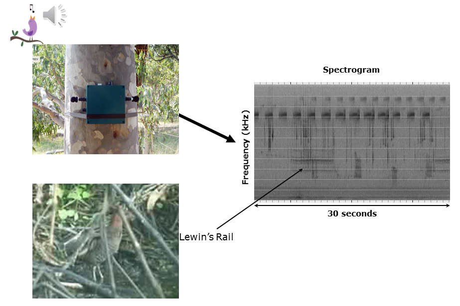
Side Note: For those new to the field, long-duration recordings obtained for ecoacoustic analysis are typically obtained from recording units attached to trees like those in the pictures above. To date, the two most commonly used recording units are Song Meters manufactured by Wildlife Acoustics, Massachusetts (above left image) or BAR recording boxes manufactured by Frontier Labs, Brisbane (above right image). An interesting and cheaper new-comer to the field is the AudioMoth.
Slide 2: So just how old is ecoacoustics?
As far as I am aware, the earliest publication describing an acoustic index used for ecological purposes is a 2001 paper from the lab of Stuart Gage. This probably makes Stuart the “founding father” of ecoacoustics. Stuart published several other papers in subsequent years, but the next new index to be published was due to Boelman in 2007. It is interesting to note that both these indices are still being used today. Another two widely used indices were published in 2008: the ACI index1 from Almo Farina’s lab and the entropy index from Jerome Sueur’s lab.

Slide 2.
The soundscape literature dates back to a seminal book by Murray Schaffer in 1994, well worth reading because it is a beautiful synthesis of sound, poetry, and science. Another influential figure in the history of soundscape recordings is Bernie Krause. And the coming together of many of these pioneers produced the 2011 paper by Pijanowski et al. Our lab, the QUT Ecoacoustics Research Group, also started publishing in 2008. Our research interest has always been to address the computational and “big data” problems presented by the accumulation of terabytes of acoustic recordings.
I like to think that, while the conception of ecoacoustics may have been in 1994 or 2001, the bumper crop of papers in 2008 dates that year as the birth of ecoacoustics. 2008 to 2018—In computing science, ten years is a long time, perhaps even three generations-worth, and enough time for a new discipline to come of age. But has it?
Slide 3: The information pyramid
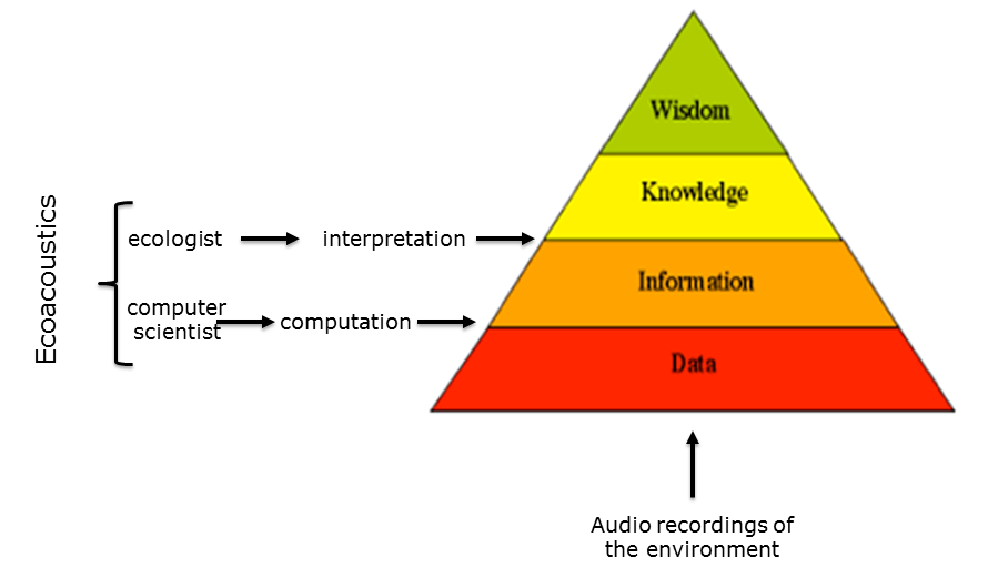
Before broaching this question, I should place some boundaries around my endeavour by referring to the well-known information pyramid. According to the pyramid, the synthesis of data produces information, the synthesis of information produces knowledge and the distillation of knowledge becomes wisdom.
Slide 3.
In the case of ecocoustics, data is mostly derived from audio recordings of the environment. The transition from data to information requires computation which is generally the work of computer scientists and the transition from information to knowledge requires interpretation which, in the case of ecocoustics, is the work of ecologists. Ecoacoustics requires the close cooperation of computer scientists and ecologists, in the same way that bioinformatics requires the interweaving of computation and biology.
So, by way of a caveat, in attempting to answer the question “Has ecoacoustics come of age?”, I admit to taking the perspective of a computer scientist.
Slide 4: The world according to ecoacoustics
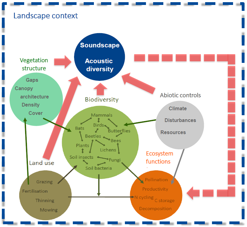
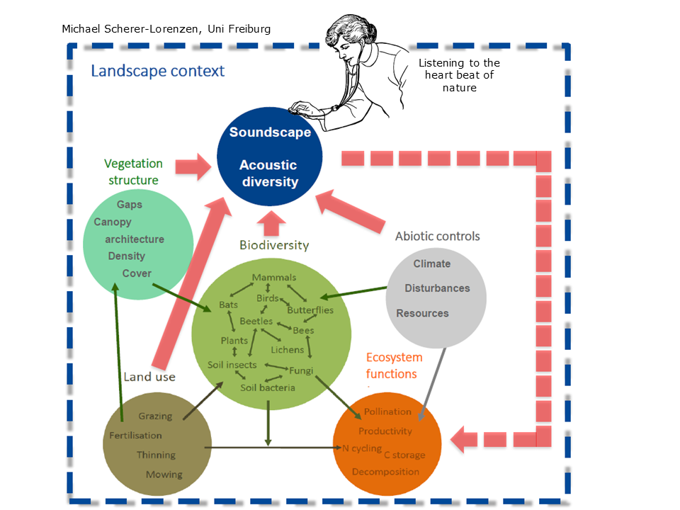
At the first Ecoacoustics Congress, Michigan State University, 2016, Michael Scherer-Lorenzen from University of Freiburg put up this slide illustrating the relationship of ecoacoustics to the larger discipline of ecology. The bottom five circles illustrate a model of the interlocking components of an ecosystem. Each of these components produces sound, the collectivity of which is the soundscape produced at a given location.
Slide 4.
The most important feature of this diagram is the dotted line from the soundscape circle returning to the bottom of the diagram. This indicates that the production of a soundscape is a dynamic system because the output of the system returns to become an input.
Slide 5: Listening to the heartbeat of Nature
Slide 5.
At the same Congress, Stuart Gage described ecoacoustics using the metaphor “listening to the heart-beat of nature”. This is an elegant metaphor because, just as a doctor listens to your heart beating, your lungs breathing and your tummy gurgling and thereby tells you more about your state of health than you wish to know, so too, ecologists can derive a great understanding of the “health” of an ecosystem by listening to the sounds it produces.
Slide 6: The standard spectrogram
I will begin to address the question motivating this talk by describing a little of the work we have been doing in the Ecoacoustics Research Group over the past few years. Some of this is a review of slides already presented in the tutorial Long-duration Audio-recordings of the Environment. My apologies for that.
Slide 6.
Ecologists have long worked with spectrograms, two dimensional representations of sound, with time as the x-axis and frequency (hertz or kilohertz) as the y-axis. Sound amplitude is encoded as a shade—the darker the shade, the more intensity. The typical spectrogram will be a few seconds long, or as long as required to demonstrate the animal call of interest. The above 30-second spectrogram illustrates the “kek-kek” call of the cryptic Lewin’s Rail. The recording was made on the outskirts of Brisbane City in 2010. The sounds at 8 kHz and above are due to crickets. There are at least four other birds calling.
Slide 7: …but the standard spectrogram does not scale!
Unfortunately, if we want to prepare a spectrogram of a 24-hour recording at similar scale to that shown in the previous slide, we would require a computer screen 1.2 kilometers wide! (“A mile a day” in USA speak!) If instead, we squeeze a 24-hour recording into a standard audio software tool such as Audacity, we end up with a smeared-looking image, like the one below. This is because Audacity averages over the recording in order to achieve the three-orders-of-magnitude compression required to squeeze it into the available space. (Warning: do not try this unless you know how to fix a constipated computer!) Averaging renders most of the acoustic structure invisible.

Slide 7.
Slide 8: Different indices - different views
In order to compress an audio recording and retain as much information as possible (that is, avoid the “smearing” problem), we can calculate a set of acoustic indices at one-minute resolution. In this example, we have taken a four-hour recording and calculated three indices at one-minute resolution: ACI, H(t), and CVR. The choice of acoustic indices is very important but outside the scope of this tutorial. Please go to the introductory tutorial Long-duration Audio-recordings of the Environment for more detail on the preparation of long-duration false-colour spectrograms. See also Towsey, 20142 and 20173 for details on the calculation of several acoustic indices that we regularly use.

Slide 8.
What is important to note in the above spectrograms is that each of the indices provides a different view of the four-hour soundscape. Acoustic indices may be compared to camera lens filters—different filters offer different views of a landscape.
Slide 9: False-colour spectrograms
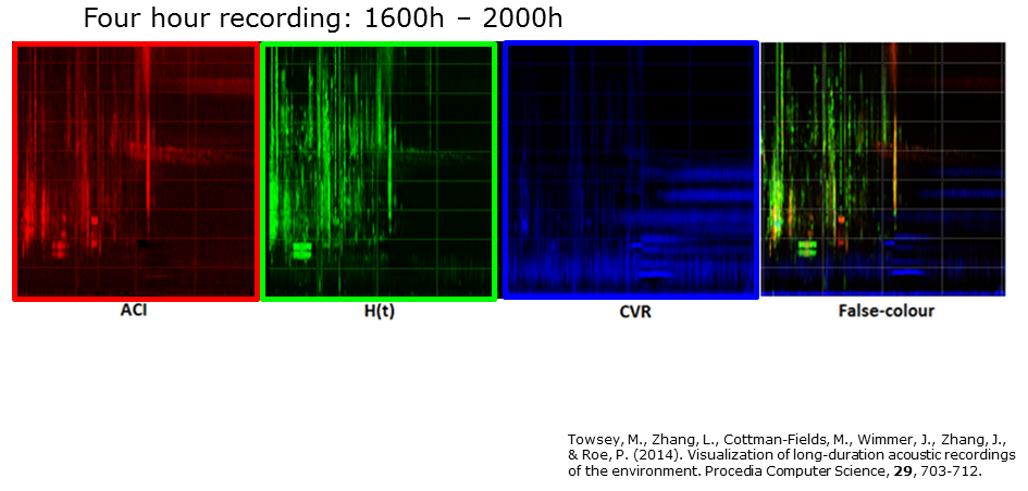
Slide 9.
The next step in the production of long-duration spectrograms was inspired by false-colour satellite imagery in which pictures of the earth’s surface are rendered in three colours by assigning the red, green, and blue (RGB) colours to sensors that respond to different parts of the electromagnetic spectrum. In this case we assign RGB to the three different spectrograms and thereby produce the long-duration false-colour (LDFC) spectrogram seen on the right-hand side of this slide. Note how much detailed structure in the sound-space is revealed.
Slide 10: The utility of 24-hour, false-colour spectrograms
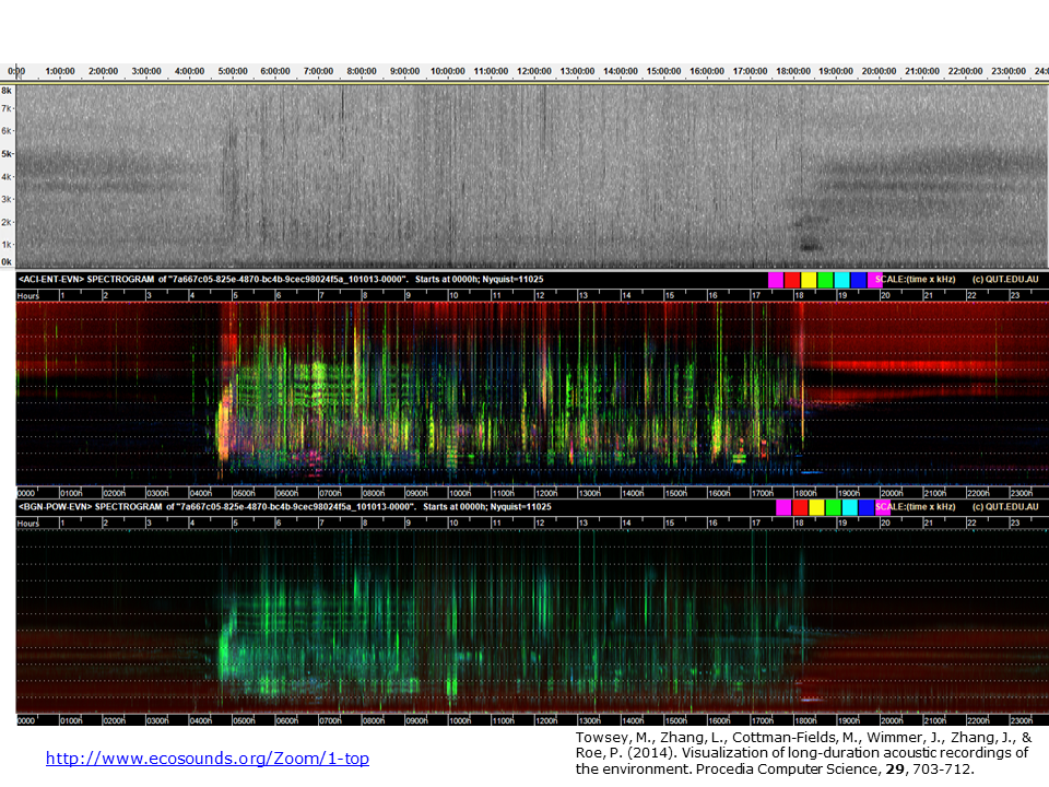
Slide 10.
Here we see how much additional acoustic structure can be seen in a false-colour spectrogram. Each of the three spectrograms is of the same 24-hour recording made in open eucalypt woodland at the Samford Ecological Research Facility on the outskirts of Brisbane city. (This is the same recording from which the four hours of the previous slide were extracted.)
Each spectrogram starts at midnight and finishes the following midnight. Midday is in the centre. The top spectrogram is the one produced by Audacity. The middle, false-colour spectrogram is produced by assigning the ACI, H(t), and CVR indices to the RGB channels respectively. The basic structure of the forest soundscape is easily interpreted. The morning chorus is clearly visible at 04:45. It tends towards white in colour where all indices have high values. The onset of evening is indicated by the appearance of acoustic tracks due to insects. But clearly there are many other events. The colours of acoustic events in the spectrogram depend both on the three indices used and on the characteristic distribution of acoustic energy in the animal call(s) that contribute to the event. With some experience you begin to recognise the different sounds of interest.
Different combinations of indices give different views of the soundscape. The bottom image is constructed from three different indices, background noise (BGN), power (POW), and event count (EVN). Note how less acoustic structure is visible in the bottom spectrogram because two of the three indices (POW and EVN) are correlated. Since these indices are assigned to the green and blue channels respectively, there is a uniformity of cyan colour representing daytime acoustic activity.
Important conclusion: the three indices used to construct an LDFC spectrogram should be minimally correlated. For more detail see previous tutorials and publications.
Slide 11: Biophony revealed in a 24-hour LDFC spectrogram
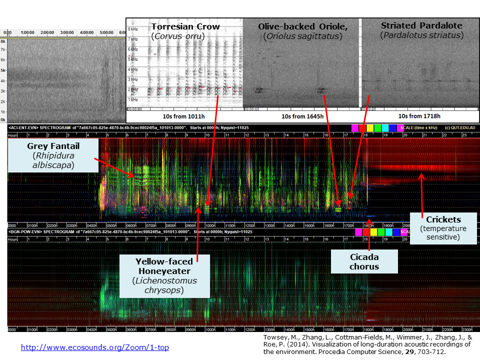
Slide 11.
In this slide, we identify some of the birds that produced the acoustic events visible in the LDFC spectrograms. A cicada chorus is visible at 800Hz, at 18:00. Note that much of the structure in these images comes about because a bird (or birds) tends to sit in the same tree for a few minutes and is likely to repeat the same song/call. Even though a bird may only call once or twice in a minute, typically at least one acoustic index will “detect” the call, and calls over consecutive minutes will leave a clearly visible trace in the spectrogram. Note that LDFC spectrograms were never designed to identify bird species. The fact that this is possible has turned out to be remarkably useful. More on this later.
You can see an interactive version of this slide here.
Slide 12: LDFC spectrograms of three sites at different latitudes

Slide 12. Top audio courtesy of Eddie Game and the Nature Conservancy. Bottom audio courtesy of David Watson (CSU)
This slide compares three 24-hour, false-colour spectrograms of three soundscapes from different latitudes. All these recordings were obtained in the first week of July (winter) 2015. The top Papua New Guinea recording is dominated by insects. It is hard to imagine squeezing more sound into this soundscape. PNG jungles are very loud. The middle recording (from Gympie National Park, about 150 kilometers north of Brisbane) is very quiet at night (because the temperatures are near freezing) and dominated by birds during the day. The bottom recording is from Sturt National Park in the far north-west corner of New South Wales, Australia. The conditions are desert-like. Not only is it very cold at night, but during the day it blows a gale (the yellow-red lines in the middle of the spectrogram). The desert morning chorus is diminutive. Soundmarks are very useful (actually essential) in order to orient oneself in a soundscape. They are the equivalent of landmarks in a landscape.
Slide 13: Comparing land-use soundscapes
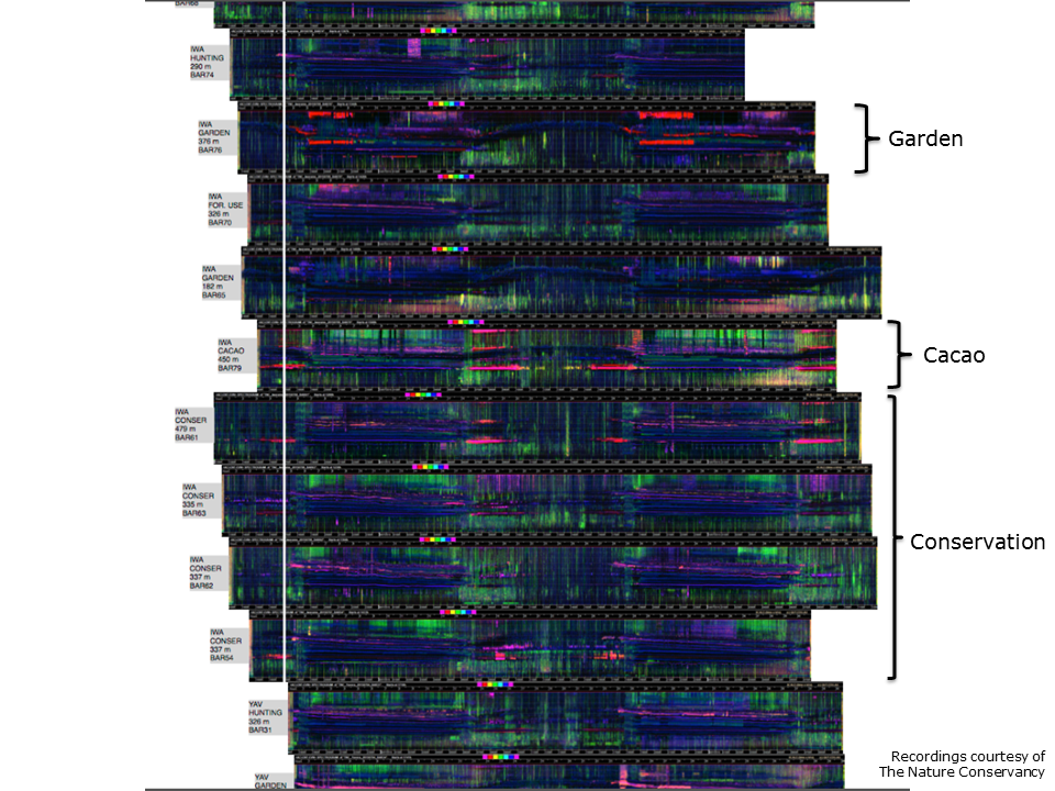
Slide 13. Audio courtesy of Eddie Game and the Nature Conservancy.
It is not very clever to distinguish a jungle soundscape from a desert soundscape—it does not require LDFC spectrograms. This technique comes into its own when comparing soundscapes for diagnostic purposes, for example, when comparing the soundscapes resulting from different land use conditions.
This slide compares the soundscapes of several sites in the Adelbert Mountains of PNG, subject to different land uses, such as conservation, gardening and cacao plantation. The 24-hour LDFC spectrograms are aligned midnight to midnight. It is easily apparent that the garden site has a different soundscape.
Note that an LDFC spectrogram is not an end in itself. Rather it facilitates the asking of further questions. An image does not easily lend itself to statistical analysis, but these LDFC spectrograms are derived from acoustic indices, which can be subject to statistical analysis.
Slide 14: Sampled recordings
Slide 14.
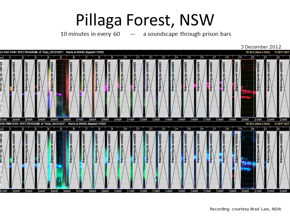
Sampled recordings do not lend themselves to useful LDFC spectrograms. In this example the recording unit was set to record 10 minutes in every hour, with a longer recording interval during the morning and evening chorus. However, note that the final recordings missed most of the morning chorus!
Slide 15: Sampled recordings
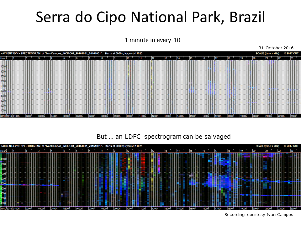
Slide 15.
You might think that recording one minute in every ten is likely to result in a worse LDFC spectrogram (top image). However, we can rescue this situation and produce a reasonable LDFC spectrogram by extending the one-minute spectrogram to fill in the nine-minute gaps (bottom image).
Important conclusion: In order to produce a useful LDFC spectrogram, it is better to record one-minute in every N minutes, as opposed to N-minutes in every half-hour or hour.
Editor’s note: only for making these particular sort of images. We still greatly prefer continuous recordings, or failing that, longer recordings!
Slide 16: Freshwater recordings
Slide 16.
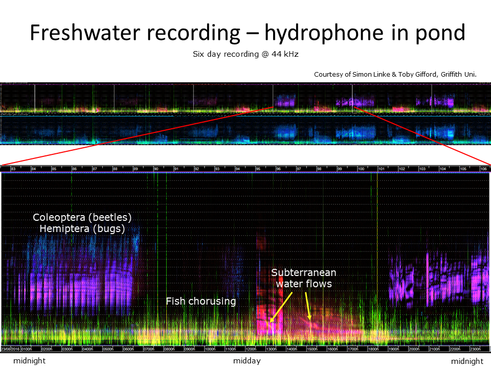
The top spectrogram shows six days of continuous recording using a hydrophone immersed in a waterhole. This waterhole is part of a chain of waterholes that join up to become a raging torrent during the Australian monsoon season. There is a surprising amount of acoustic activity in this isolated pool, mostly due to insects and fish. There is other acoustic activity however, due to movement of water through underground channels. A single day of recording has been enlarged (bottom image) to reveal more detail.
This six-day spectrogram has another purpose—to demonstrate that LDFC spectrograms are not useful for illustrating recordings more than a day or two in length. Another visualisation technique is required.
Slide 17: Ribbon plots

Slide 17.
To visualise many consecutive days of recording we use stacked ribbon plots. A 24-hour LDFC spectrogram is reduced to a height of 32 pixels but retains its full 24-hour width. This image illustrates 30 days of continuous recording from Gympie National Park, November 2015. The site consists of open Eucalypt woodland on a well drained site (see inset). The morning chorus is clearly visible from day to day as are periods of heavy rain rendered in red/orange.
Slide 18: Large-scale acoustic structure

Slide 18.
This image magnifies a few days of morning chorus from the previous image. Note how the first four morning choruses have a similar temporal structure, which reflects the differing arrival times of bird species to the morning chorus. Stacked ribbon plots are useful because they reveal long-term changes in patterns of acoustic structure, that is, over weeks and months.
Slide 19: Marine recordings
Slide 19
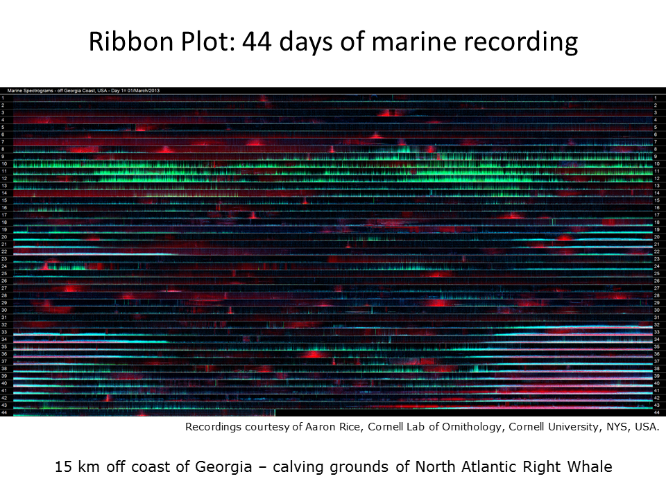
This stacked ribbon plot is derived from 44 days of marine hydrophone recording taken 15 km off the coast of Georgia, USA. The water is only 15 m deep and the hydrophone was positioned 2m off the ocean floor. Note in this case, that the full-scale frequency range is only 1000 Hz. The red events are due to passing ships. The direction, speed and proximity of each ship can be determined by the shape and extension of its “red pyramid signature”.
The second dominating component of this soundscape is the cyan-blue acoustic events at night from day 33 onwards. These are due to chorusing of the black drum fish. Because of their low frequency, calls of the black drum fish carry a great distance, even 15 kilometres towards the coast.
The third dominating component of this sound-scape occurs during days 9–13. The green lines are due to unidentified “knocking” sounds. At first we thought it might be due to something hitting or biting the hydrophone. However, there were no hurricanes or other meteorological events before or during days 9–13 that might explain these acoustic events. To get a better understanding, we can add other annotations to the spectrograms as in the next slide.
Slide 20: Marine recordings
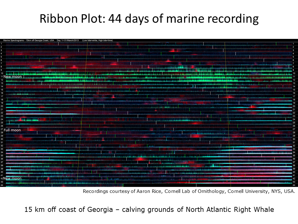
Slide 20.
This is the same 44 days of recording shown in the previous slide but with sunrise, sunset, high and low-tide times superimposed. Day length is increasing as the recording proceeds through spring. While the chorusing of black drum fish is dominant at night and likely to be triggered by increasing day-length, the chorusing does not appear to be constrained by daylight. With respect to the “knocking” sounds in days 9–13, they appear to be at a maximum between low tide and high tide around the new moon, possibly when coastal currents are strongest. We have still not been able to identify the cause of this sound, but a likely culprit is strumming of the cables tethering the hydrophone to the ocean floor due to tidal currents—a timely reminder that not all sounds in an environmental recording have a biological explanation.
It is worth noting that these hundreds of hours of marine recording were made in order to detect the presence of the North Atlantic Right Whale (NARW), the most threatened of the whale species. The hydrophone was located in the middle of the NARW calving grounds towards the end of the calving season. The usual approach is to identify NARW calls using custom computer programs. Due to the highly specific purpose of automated recognisers, they are specially designed not to detect any other acoustic events.
As it turned out, there were no whale calls in these 44 days of recording. If all you have is a whale call detector and there are no whales, the ecologist is “blind”—or perhaps “deaf” is a better description. However, LDFC spectrograms reveal a wealth of additional information about the marine soundscape. They complement the information obtained by automated call recognisers because they reveal, in much more detail, the acoustic environment in which whales live.
Slide 21: Data reduction
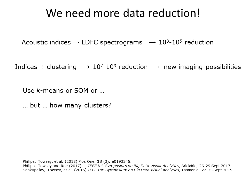
Slide 21.
Even with the ribbon spectrograms reduced to a height of 32 pixels (as in the previous slides), there is a limit to how many ribbons can be stacked to illustrate many months of recording. We need more data reduction!
LDFC spectrograms give us a 103–104 data reduction. If instead, we cluster vectors of summary indices, we can achieve a data reduction of 107–109. And this opens up many new imaging possibilities. But note that frequency information is now lost. We use k-means4 or self-organising maps5 for clustering. (See references for more details.) A big question is, how many clusters?
Slide 22: The answer: 60 acoustic clusters
60 clusters were required to obtain good discrimination of the various sources of biophony in the two years of recording that we studied. (See reference for more detail4) In order to determine what was in the 60 clusters, we listened to 20 one-minute recordings from each cluster. Although this took more than 20 hours of listening effort, it represents only a 0.1% sample of the total audio. And here we face a major challenge with long-duration audio. It is extremely difficult to ground truth by listening to sufficient audio.
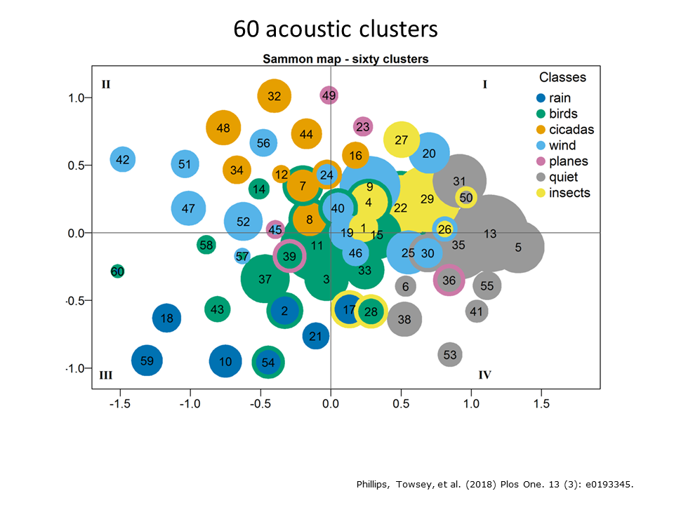
Slide 22.
To ensure that the 60 clusters made acoustic sense we projected the cluster centroids onto two-dimensions using a Sammon map. In the Sammon map shown here, the relative size of the 60 clusters is indicated by size of each circle and circle colour codes for the dominant acoustic content in each cluster. We observe that bird clusters lie close together, quiet clusters lie close together, etc. In other words, the clusters appear to make good “acoustic sense”.
Slide 23: The clusters have an ecological interpretation
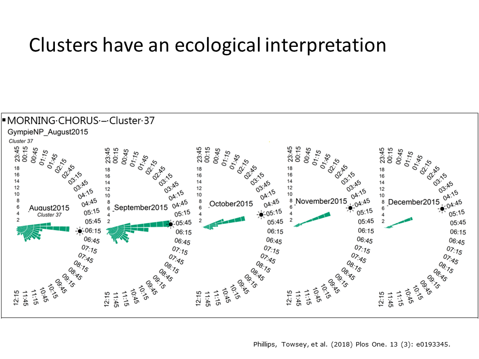
Slide 23.
The clusters also appear to have sensible ecological interpretations. Here we see plots of the occurrence of cluster 37 over the months August to December as spring transitions into summer. Note that this cluster is most abundant in spring and that its maximum tracks the sunrise as the sun rises earlier and earlier through spring and early summer. We called this the morning chorus cluster and listening to samples of it confirmed much bird calling activity.
Slide 24: The clusters have an ecological interpretation
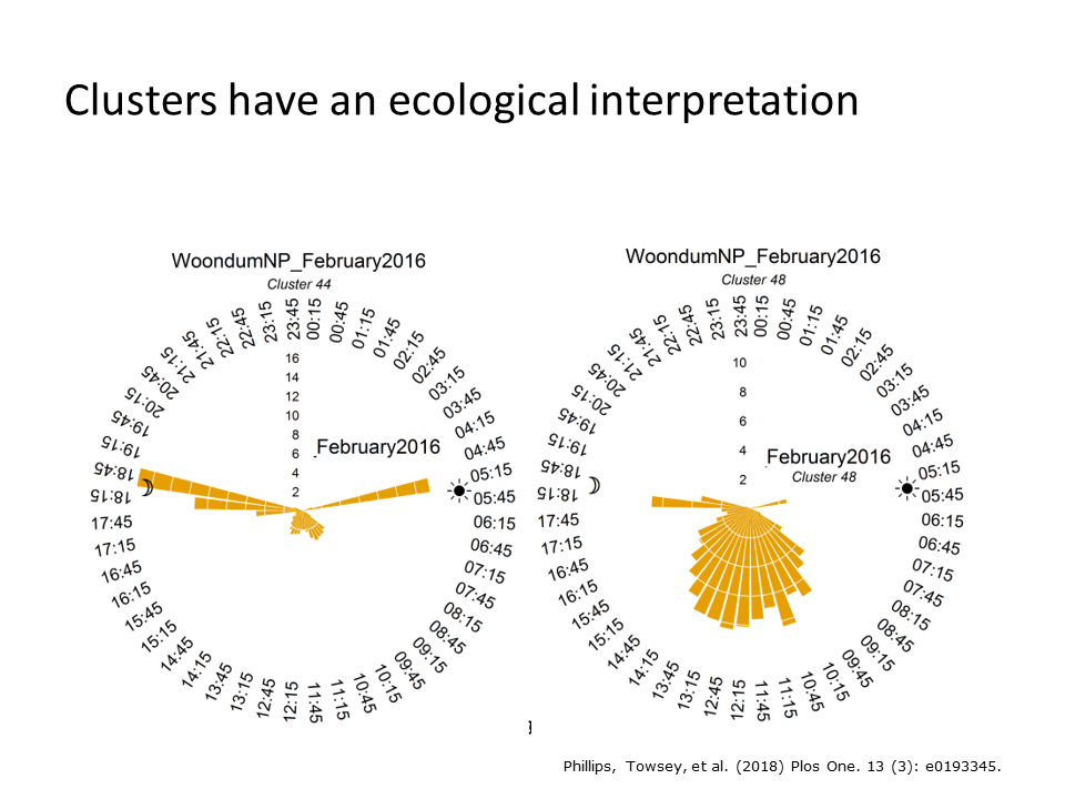
Slide 24.
This slide reveals the temporal occurrence of clusters 44 and 48 in the peak of summer. Cluster 44 coincides with sunrise and sunset, whereas cluster 48 is dominant around middle of the day. It was not difficult to establish that these clusters were due to different species of cicada chorusing.
Slide 25: Introducing Diel plots

Slide 25.
Although 60 clusters are required to discriminate the various kinds of biophony at this Eucalypt woodland site, it is difficult to colour code them with 60 colours. Therefore Phillips et al. (2018)6 colour coded the clusters according to seven basic sound categories or acoustic states as shown in the previous Sammon map: 1. silence clusters are represented in grey; 2. bird cluster in green; 3. rain clusters in dark blue; 4. wind clusters in pale blue; 5. insect cluster in yellow; 6. cicada chorus clusters in orange; and 7. plane sounds in red.
We can now prepare a diel plot in which each row of pixels (1440 pixels wide, one pixel per minute) represents a single day of sound and the total image represents 13 months of recording. Note how the soundscape changes through the seasons.
Slide 26: Diel plots
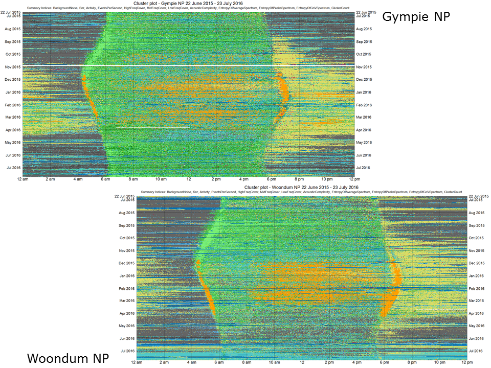
Diel plots enable us to make meaningful comparisons between the year-long soundscapes at two locations. For example, consider the two locations shown in this slide. Woondum National Park (bottom right) has higher rainfall and smaller temperature fluctuations than Gympie National Park (top left) because it is closer to the coast. Consequently, the Woondum site supports more dense vegetation cover, yet the bird species are quite similar at the two sites.
Slide 26.
Despite similar bird species, these diel plots illustrate that the soundscapes may be similar but have subtle differences. For example, the Gympie site has less cicada activity but more insect activity. We believe that images such as these will be very useful in monitoring the long term effects of climate change. Small but subtle changes in species diversity and ecosystem health will be more likely detected when very-long-duration recordings can be compared visually over consecutive years.
Slide 27:
Slide 27.
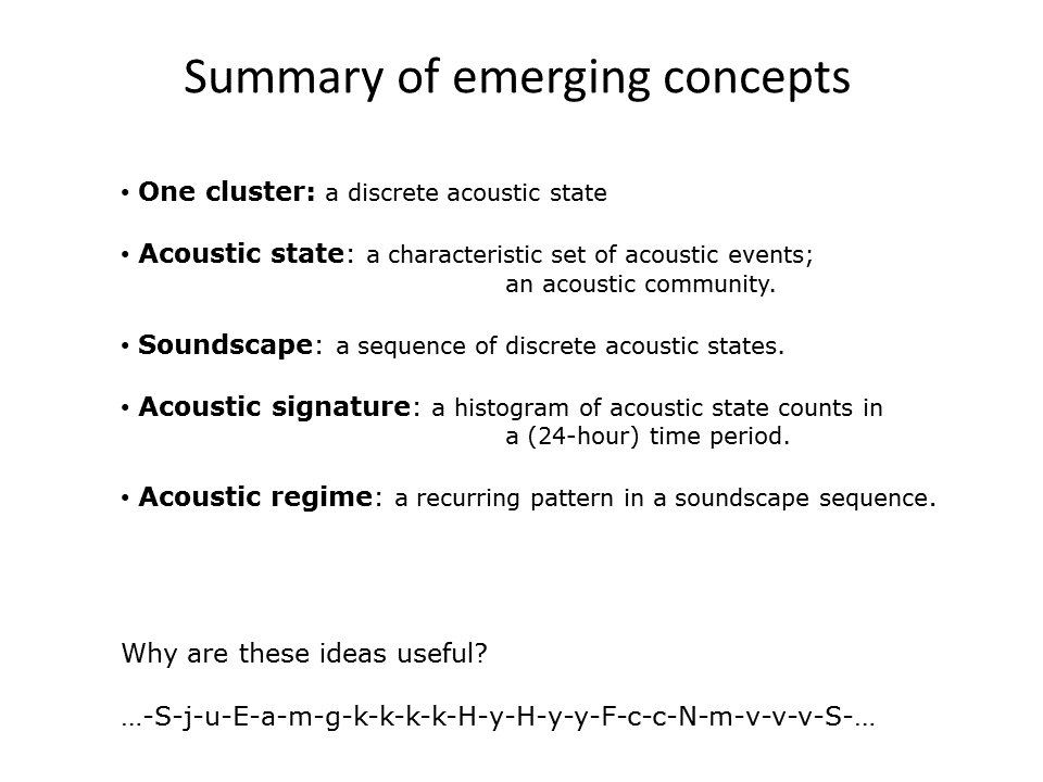
As a result of this approach to analysing long-duration acoustic recordings, several interesting concepts have emerged.
1: We consider each cluster to represent a discrete environmental acoustic state. An acoustic state in turn is a characteristic combination of acoustic events and frequently it represents an acoustic community, that is, an aggregation of species that produces sound at the same time.
2: A soundscape now becomes a sequence of discrete acoustic states.
3: Over a discrete period of time, such as a 24-hour day, a soundscape can be represented by an acoustic signature, for example, a frequency histogram of acoustic state occurrences. This has proved to be a very useful technique for us.
4: We identify recurring patterns within a soundscape sequence as acoustic regimes.
Question: What is the value of these concepts?
Answer: Representing a soundscape as a sequence of discrete states (each of which can be given a unique identifying alphanumeric symbol) is similar to representing a protein as a sequence of amino-acids (each of which is given its unique alphabetic symbol). This opens up the possibility of analysing soundscapes using the great array of bioinformatic software used to analyse amino-acid sequences.
Slide 28: Taking advantage of bioinformatic software …
Slide 28.
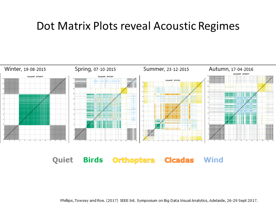
Well, it seemed like a good idea at the time! But so far, only dot-matrix plots (as shown in this slide) have proved to be useful. Here we see four days of audio, a representative day from each season, illustrated using dot-matrix plots. The soundscape sequence itself is the rising diagonal line, starting at midnight and ending the following midnight. Dot matrix plots clarify the daily acoustic structure. Winter days have a clear diurnal pattern because nights are very cold and days are dominated by birds. Spring ushers in a strong morning chorus and the intervention of insect chorusing, which reaches its peak in summer. Autumn see the gradual return to a diurnal acoustic structure.
Slide 29: The effect of different feature sets
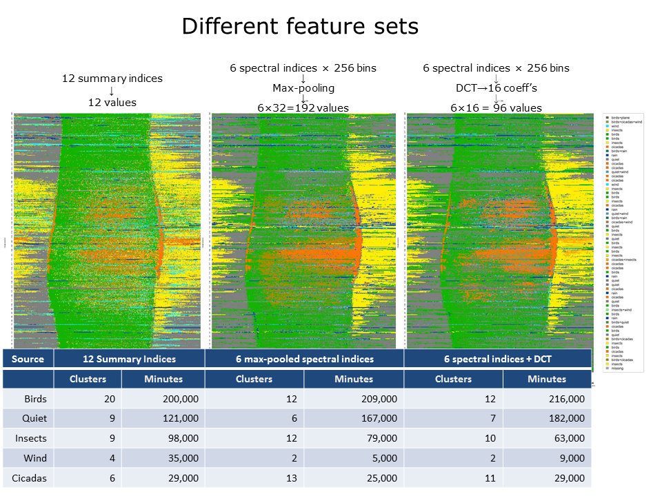
Slide 29.
To obtain the diel plots in slides 25 and 26, we clustered vectors of 12 summary indices. The question arises: would we obtain quite different results if we used a different feature set? To check this, we also clustered two other feature sets derived from exactly the same recordings: 1: Six spectral indices reduced from 256 values to 32 values by max-pooling to yield feature vectors consisting of 63×32=192 values; 2: The same six spectral indices subject to discrete cosine transforms (taking the first 16 coefficients of each) to yield feature vectors consisting of 63×16=96 values.
Following k-means clustering, the resulting 60 clusters in each case were colour coded according to their acoustic content and diel plots prepared as before. As shown in this slide, there are broad similarities between the diel plots but also significant differences.
Below the diel plots is a table giving the number of clusters and number of minutes assigned to each acoustic class. Note, for example, that while the number of bird clusters drops by almost half, the number of minutes labelled as birds remains similar. It is significant that six of the twelve summary indices used in the first feature set are derived from the 1–8 kHz band in which birds are predominant, whereas the other two feature sets are derived from the full frequency band. In other words, by deriving more features from the 1–8 kHz band, clustering has partitioned more bird clusters although the total number of instances in those clusters has not much changed.
Another difference appears to be the transfer of minutes from wind to quiet clusters. This is understandable because there is a continuous gradient from wind to quiet and a different feature set can be expected to place the partition differently.
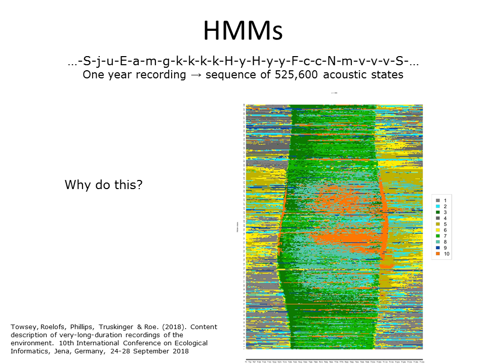
Slide 30: Deriving diel plots from HMMs
In the previous diel plot, we colour-coded the 60 clusters by listening to the medoid instance (the one-minute instance closest to the centroid) of each cluster. Another way to prepare a diel plot is to take the year long sequence of discrete acoustic states and train a Hidden Markov Model (HMM) using the forwards-backwards algorithm. The hidden states can then be colour-coded. How many hidden states? Although, in theory, the Bayesian Information Criterion should be able to tell us this, in practice it does not work well. So we explored a number of values and settled on ten hidden states as shown in the above plot.
Slide 30.
Question: Why would we want to do this?
Answer 1: 60 clusters is too many for convenient visualisation. Training an HMM reduces the cluster count.
Answer 2: Training an HMM allows sequence information to be incorporated into the derived clusters. This hope that this might facilitate the identification of underlying acoustic communities.
Answer 3: More fine-grained clustering is achieved by dividing up each cluster according to the hidden state(s) from which it is emitted.
Slide 31: Speech processing versus soundscape processing
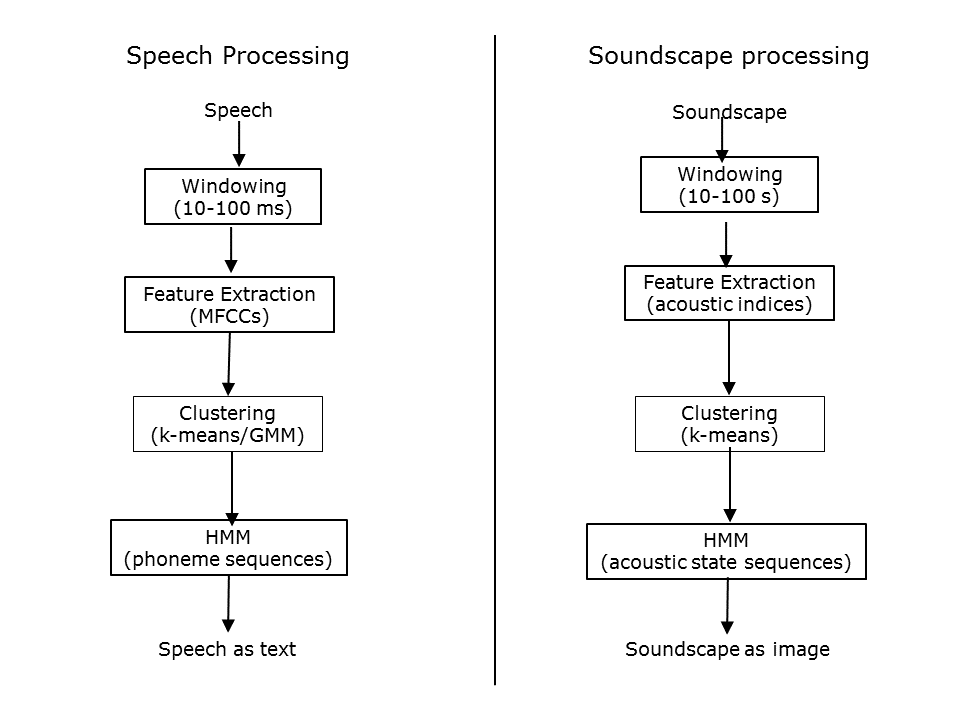
In the development of ecoacoustics to date, signal processing techniques used for speech recognition have not played a role, even though they have been used in bioacoustics studies. Perhaps these methods were not thought to be relevant at the temporal scale of ecoacoustics. This slide compares typical steps for speech processing with the steps described in the previous slides for soundscape processing. Note the similarity.
Slide 31.
Important differences are:
- the windowing time scale is 3 orders of magnitude larger for soundscape processing.
- the acoustic features appropriate for speech processing are not necessarily appropriate for the larger time-scale of soundscape processing.
- HMMs are being used quite differently in the two examples.
Nevertheless, I believe that rethinking soundscape processing in this way will help to advance the discipline of ecoacoustics by incorporating and adapting well-developed signal processing methods.
Slide 32: Coming of age?
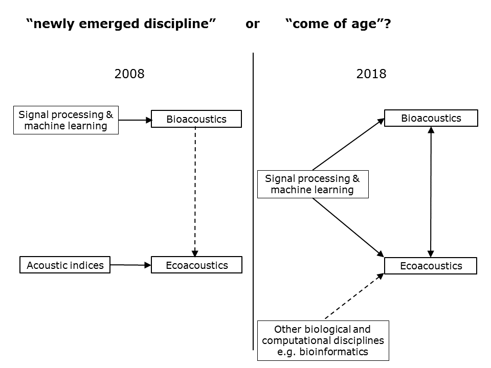
And so we return to the motivating question of this talk—is ecoacoustics still a “newly emerged discipline” or has it “come of age”? This slide, compares my understanding of ecoacoustics (from a computational perspective) in 2008 and today in 2018.
Slide 32.
In 2008, the ecoacoustics discipline was almost entirely focused on acoustic indices for its computational foundation. Meanwhile, bioacoustics had long embraced advanced signal processing methodologies. This was easy, because the timescales were similar. Another “difficulty” in 2008 (at least for me) was the uncertain relationship between bioacoustics and ecoacoustics. Almost half the presentations at the 2014 Paris conference appeared to lie in the realm of bioacoustics rather than ecoacoustics. But I was new to the field and still coming to terms with its topography.
In 2018, I believe we can say that ecoacoustics has come of age. Some significant developments are:
1: Acoustic indices are no longer treated as having some special ecological significance. They are simply acoustic features that are useful only to the extent that they help to highlight acoustic phenomena of interest.
2: Ecoacoustics is now in a position to embrace the concepts and methodologies of signal processing at larger timescales.
3: Ecoacoustics is increasingly integrated into the overlapping interests of other biological and computational disciplines. For example, it is in a position to utilise the computational software of other disciplines, especially bioinformatics.
4: And finally, There is a recognition that there are a continuum of valid questions from bioacoustics to ecoacoustics. May be that was always the case, but it is a new thought for me and…
…I would like to devote the rest of this talk to scanning the spectrum from bioacoustics to ecoacoustics.
Slide 33: Bridging the gap
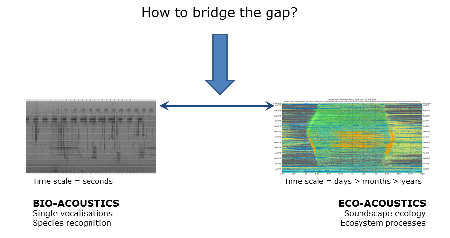
Slide 33.
When we originally developed LDFC spectrograms, the intention was merely to facilitate the navigation and interrogation of long-duration recordings that could not be easily opened using software such as Audacity. We did not expect that the technique would be useful to identify individual species but it has turned out to be so.
Slide 34: Frog chorusing
While an individual frog call may last only a fraction of a second, frog chorusing and indeed the chorusing of many animals can last from minutes to hours. This brings chorusing into the ecoacoustics timescale and means it is amenable to ecoacoustic techniques.
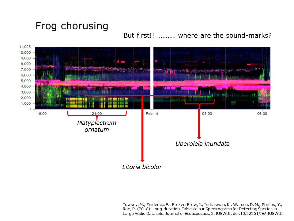
Slide 34.
This slide displays a 12-hour night-time false-colour spectrogram that includes the chorusing activity of three frog species (see labels). But you should also be aware of the soundmarks in this image.
- Can you identify, the morning and evening chorus?
- What is that pink line at 4500 Hz?
- Why is the pink line at 7500 Hz descending slightly?
The take-home message is that the starts and ends of chorusing behaviour can be clearly identified using combinations of acoustic indices in LDFC spectrograms.
Slide 35: Detecting cane-toads

Slide 35.
Likewise, the long-duration calling of the cane toad can be easily detected in LDFC spectrograms. At the bottom of this LDFC spectrogram is the output of a custom built cane toad recogniser. It has clearly picked up the cane toad—but it was a lot more work to write the custom recogniser than to use the generic features of the LDFC spectrogram.
Slide 36: Detecting cryptic species
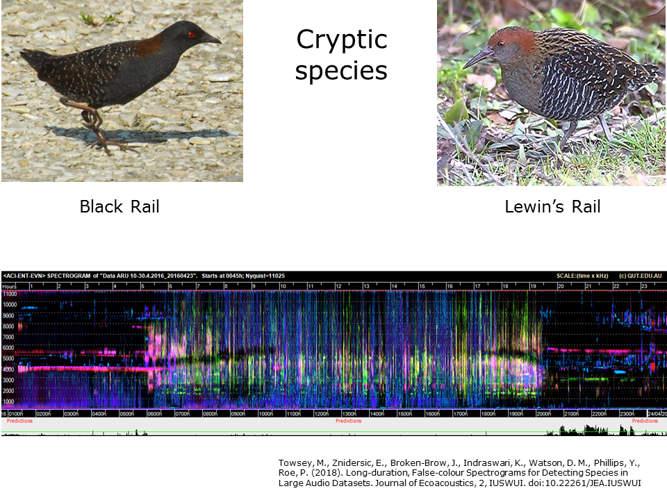
Slide 36.
Perhaps the biggest surprise we have had in the QUT Ecoacoustics group recently is the usefulness of generic acoustic indies in detecting cryptic and/or threatened bird species such as the Lewin’s Rail, Black Rail, Least Bittern, and Bhutanese White Heron.
The advantages of this technique are: 1: Compressed timescale; 2: Generic features; 3: get soundscape + species detection
- Faster preparation of datasets because of labelling at low resolution low resolution, i.e. one label per one minute.
- Faster preparation of recognisers because of using generic indices.
- Get both soundscape visualisation and species recogniser in the same processing steps.
- Visual scanning of the LDFC spectrograms allows for fast checking of false-positive and negatives and has led to the discovery of new species for a given location.
These advantages come with a serious limitation—the species of interest is only detected where its calls are the dominant acoustic activity in its frequency band over the minute. Surprisingly, the technique has proved to be extremely useful, despite this limitation.
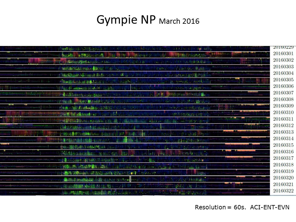
Slide 37: Detecting bats
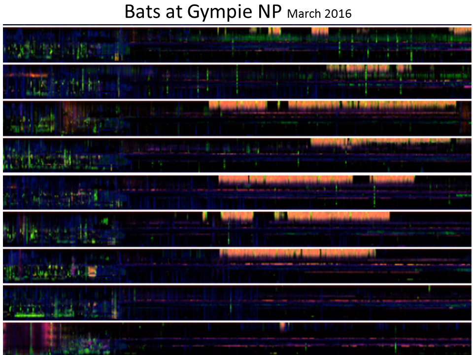
Given the low resolution of the LDFC technique as originally developed we had no expectation that would prove useful for identification of echolocating micro-bats. However, we noticed the “red/orange” events in the late evening of several days in March 2016 (see the below stacked ribbon plot) and eventually identified the source as the white-striped free-tailed bat.
 <figcaption style="margin-top: 0.3em" class="text-muted small">
<p>Slide 37.</p>
</figcaption>
<figcaption style="margin-top: 0.3em" class="text-muted small">
<p>Slide 37.</p>
</figcaption>
Slide 38: Detecting bats
Here is the same bat call in more detail. This bat is unusual in that the lower range of its call is below the Nyquist of 11025 Hz that we typically use for LDFC spectrograms.
Slide 38.
Slide 39: Detecting bats
Slide 39.
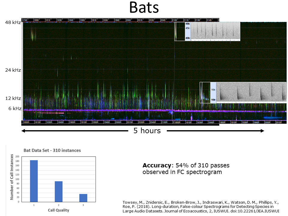
In another set of night-time recordings using SM4 recording units at their maximum sampling rate of 96 kHz (Nyquist = 48 khz), we could detect all four species of bat present in those recordings. The above LDFC spectrogram shows the traces of the bat calls and what they look like in standard scale spectrograms. We were able to detect 54% of the 310 echolocation passes. This detection rate may seem low, but it is to be remembered that the majority of the passes consisted of low quality calls (see inset, bottom left).
Another new feature of this LDFC spectrogram is that the generic indices were calculated at 15 second resolution rather than 60 second resolution.
Slide 40: Zooming spectrograms
Slide 40.
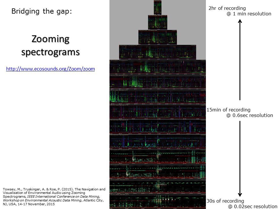
In previous slides, we have demonstrated the use of acoustic indices calculated at one-minute resolution (and 15 second in case of previous slide). The resolution of a standard spectrogram (as seen for example, in Slide 6) is around 0.01 seconds per frame. In fact it is possible to calculate acoustic indices at multiple time scales and use them to span the entire temporal scale from years and months down to milliseconds. Some indices reveal acoustic structure better at course resolution (for example ACI) and others reveal structure better at fine resolution. We are able to “stitch” all these different scale images together to make a pyramid stack as shown in the above slide. But much more useful is that we are now able to “zoom” in and out of long duration recordings in the same way that Google Maps allows you to zoom in and out from planet Earth. This makes it easy to navigate recordings of arbitrary duration. Try a demo of this concept for yourself on a 24-hour recording by going to http://www.ecosounds.org/Zoom/zoom.
We have integrated the zooming false-colour spectrograms technology into our acoustic workbench software 7.
Slide 41: Calculating acoustic indices at higher resolution
Slide 41.
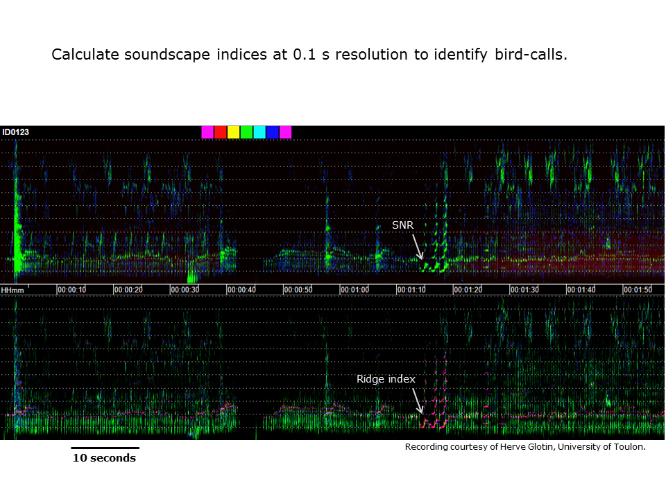
As we cross the spectrum from ecoacoustics to bioacoustics we reach a point where it is possible to calculate generic acoustic indices at 0.1 second resolution. This slide illustrates the use of six acoustic indices to visualise the calls of a European song bird.
Slide 42: The future of soundscape processing
To conclude this talk, just a few brief words about the future of ecoacoustics.
- As pointed out by Craig Radford at this 2018 Congress, we require broadly accepted protocols for the recording, storage, analysis and reporting of long duration recordings of the environment.
- It will require an ongoing research effort to develop new acoustic features that inform ecological studies.
- The content description of long-duration recordings of the environment will be a useful development because this will take advantage of the highly efficient search capabilities of text databases.
But of course we must never forget that the final purpose of advances in computational ecoacoustics is to assist ecologists with the interpretation of long-duration recordings of the environment.
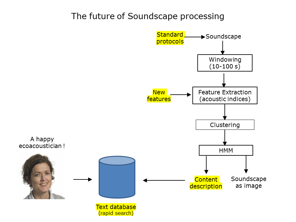
Slide 42.
References
-
N. Pieretti, A. Farina, D. Morri (2011). A new methodology to infer the singing activity of an avian community: The Acoustic Complexity Index (ACI), Ecological Indicators, Volume 11, Issue 3, May 2011, Pages 868-873, ISSN 1470-160X, http://dx.doi.org/10.1016/j.ecolind.2010.11.005. ↩
-
Towsey, M. et al., (2014). Visualization of long-duration acoustic recordings of the environment. Proceedings of the International Conference on Computational Science (ICCS 2014), Cairns, Australia, 9-12 June 2014, http://dx.doi.org/10.1016/j.procs.2014.05.063. ↩
-
Towsey, M. (2017) The calculation of acoustic indices derived from long-duration recordings of the natural environment. QUT ePrints, Brisbane, Australia. https://eprints.qut.edu.au/110634. ↩
-
Phillips, Y., Towsey, M., and Roe, P. (2017, 6-10 November). Visualisation of environmental audio using ribbon plots and acoustic state sequences. Paper presented at the IEEE International Symposium on Big Data Visual Analytics (BDVA), Adelaide, Australia. doi:10.1109/bdva.2017.8114628. ↩ ↩2
-
Sankupellay, Mangalam, Towsey, Michael W., Truskinger, Anthony, & Roe, Paul (2015) Visual fingerprints of the acoustic environment: The use of acoustic indices to characterise natural habitats. In IEEE International Symposium on Big Data Visual Analytics (BDVA 2015), 22-25 September 2015, Hobart, Tas, http://dx.doi.org/10.1109/BDVA.2015.7314306. ↩
-
Phillips, Y. F., Towsey, M., & Roe, P. (2018). Revealing the ecological content of long-duration audio-recordings of the environment through clustering and visualisation. PLoS ONE, 13(3), e0193345. https://doi.org/10.1371/journal.pone.0193345 ↩
-
Towsey, M., Truskinger, A. & Roe, P. (2015). The Navigation and Visualisation of Environmental Audio using Zooming Spectrograms. IEEE International Conference on Data Mining, Workshop on Environmental Acoustic Data Mining, Atlantic City, NJ, USA, 14-17 November, 2015, http://eprints.qut.edu.au/91822/. ↩